Imagine you are driving an EV. The dashboard screen shows a comforting 15% State of Charge (SOC)plenty of range to reach the next charging station. Then, suddenly, the powertrain loses power and the car shuts down.
In the BMS world, this is the ultimate nightmare. It’s the result of inaccurate State of Charge (SOC) estimation.
Calculating how much energy is left in a lithium-ion battery isn't like measuring fuel in a gas tank. There is no physical float sensor inside the cell. Instead, we must infer the inner state of a complex, non-linear chemical reactor using only three external inputs: voltage, current, and temperature.
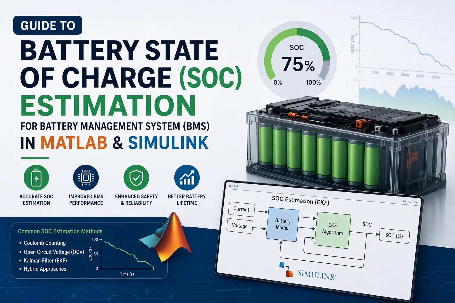
If you are building a Battery Management System (BMS) in MATLAB or Simulink, this guide will walk you through the practical engineering workflows to get SOC estimation right.
The Hard Truth About SOC Methods: From Simple to Production-Grade
1. Coulomb Counting (Ah Integration)
At its core, Coulomb counting is bookkeeping. You measure the current flowing in and out of the battery and integrate it over time:
SOC(t) = SOC(t0) - (1 / (3600 * Q_nominal)) * integral_t0_to_t( I(tau) d_tau )
The Trap: Current sensors have offsets. Even a tiny 10mA calibration error will accumulate over a 4-hour drive, causing your SOC estimate to drift significantly. If your initial SOC estimate is wrong, Coulomb counting has no way of correcting itself.
2. Open Circuit Voltage (OCV) Lookup
Every battery chemistry has a unique relationship between its resting voltage and its SOC.
The Trap: To measure Open Circuit Voltage, the battery must be at rest (no current flowing) for hours to let the internal chemistry stabilize. Under dynamic load, terminal voltage drops due to internal resistance and polarization. If you use terminal voltage under load to estimate SOC, your estimate will fluctuate wildly every time the driver hits the accelerator.
3. Extended Kalman Filter (EKF)
This is the production standard. EKF combines the math of Coulomb counting with a physics-based Equivalent Circuit Model (ECM) of the battery.
It runs a real-time simulation of the battery model inside the BMS microcontroller. If the model's predicted terminal voltage disagrees with the physically measured terminal voltage, the Kalman gain corrects the internal SOC state. It constantly corrects for sensor drift and bad initial assumptions.
Walkthrough 1: Using Simscape Battery Estimator Blocks
If you are using MathWorks' Simscape Battery library, you don't need to write Kalman filter algorithms from scratch.
The Implementation Workflow:
1. Define your cell model: Drag a Battery (Table-Based) block into your Simulink canvas. Configure its parameters (capacitance, resistance, OCV-SOC lookup tables) based on your cell manufacturer’s data sheet.
2. Apply a load profile: Connect a Controlled Current Source representing a drive cycle (e.g., UDDS or US06) to discharge the battery model.
3. Place the Estimator:Search for the SOC Estimator (Kalman Filter) block in the Library Browser (Simscape > Battery > BMS > Estimators).
4. Wire the Inputs: Connect the measured terminal voltage, current, and cell temperature to the estimator block.
5. Configure the Estimator: Double-click the block and select Extended Kalman Filter (EKF). Input your battery parameter tables (OCV, R0, R1, C1) directly into the block UI.
6. Run and Compare: Open the Simulation Data Inspector to plot the "True SOC" from the Simscape Battery block against the "Estimated SOC" from the estimator.
Walkthrough 2: Writing a Custom EKF in MATLAB
For specialized applications or if you want to understand the underlying math, writing a custom EKF in a MATLAB Function block is a great exercise.
Here is a clean, runnable MATLAB class that implements a first-order equivalent circuit model (one RC branch) inside an EKF loop:
classdef BatteryEKF < handle
properties
% Battery Parameters
Q_nom = 3600 * 3.0; % Capacity in Ampere-seconds (3.0 Ah cell)
R0 = 0.02; % Ohmic resistance (Ohms)
R1 = 0.015; % Polarization resistance (Ohms)
C1 = 2000; % Polarization capacitance (Farads)
dt = 0.1; % Time step (seconds)
% OCV lookup parameters (linearized for demonstration)
% In production, replace with a spline or polynomial lookup
ocv_soc_grid = [0.0, 0.1, 0.2, 0.3, 0.4, 0.5, 0.6, 0.7, 0.8, 0.9, 1.0];
ocv_val_grid = [3.0, 3.4, 3.5, 3.6, 3.7, 3.8, 3.9, 4.0, 4.1, 4.15, 4.2];
% Filter States
x = [0.8; 0]; % State vector: [SOC; V1] (Initial SOC = 80%)
P = diag([1e-4, 1e-4]); % State covariance matrix
Q = diag([1e-6, 1e-6]); % Process noise covariance
R = 1e-3; % Measurement noise covariance (voltage sensor noise)
end
methods
function soc = step(obj, current, v_meas)
% current: Positive for discharge, negative for charge
% v_meas: Measured terminal voltage (V)
% 1. Predict Step (Model Propagation)
soc_prev = obj.x(1);
v1_prev = obj.x(2);
% State transition matrices
A = [1, 0; 0, exp(-obj.dt / (obj.R1 * obj.C1))];
B = [-obj.dt / obj.Q_nom; obj.R1 * (1 - exp(-obj.dt / (obj.R1 * obj.C1)))];
% Predict states
x_pred = A * obj.x + B * current;
% Predict covariance
P_pred = A * obj.P * A' + obj.Q;
% 2. Update Step (Correction using Voltage Measurement)
soc_pred = x_pred(1);
v1_pred = x_pred(2);
% Calculate OCV and its derivative d(OCV)/d(SOC) at predicted SOC
ocv = interp1(obj.ocv_soc_grid, obj.ocv_val_grid, soc_pred, 'linear', 'extrap');
% Compute Jacobian H = [d(V_terminal)/d(SOC), d(V_terminal)/d(V1)]
% V_terminal = OCV(SOC) - V1 - I * R0
h_soc = (interp1(obj.ocv_soc_grid, obj.ocv_val_grid, soc_pred + 0.001, 'linear', 'extrap') - ...
interp1(obj.ocv_soc_grid, obj.ocv_val_grid, soc_pred - 0.001, 'linear', 'extrap')) / 0.002;
H = [h_soc, -1];
% Compute predicted terminal voltage
v_pred = ocv - v1_pred - current * obj.R0;
% Innovation (Measurement Residual)
y = v_meas - v_pred;
% Kalman Gain
S = H * P_pred * H' + obj.R;
K = (P_pred * H') / S;
% Update State and Covariance
obj.x = x_pred + K * y;
obj.P = (eye(2) - K * H) * P_pred;
% Ensure SOC remains bounded between 0 and 1
obj.x(1) = max(0, min(1, obj.x(1)));
soc = obj.x(1);
end
end
end
3 Lessons From the Field: What the Textbooks Leave Out.
If you want your BMS code to run reliably on real microcontrollers under real driving conditions, keep these three lessons in mind:
1. The Q and R Tuning Headache
Tuning the process noise covariance matrix (Q) and measurement noise covariance matrix (R) is where most engineers get stuck.
- If R is too high, the filter ignores voltage feedback, reverting to drifting Coulomb counting.
- If Q is too high, the filter chases sensor noise, causing the estimated SOC to bounce around erratically.
- Solution: Collect clean lab data of a cell experiencing white-noise voltage readings under no load to establish a baseline for R.
2. Hysteresis in LFP Batteries
Lithium Iron Phosphate (LFP) cells have an extremely flat OCV curve. Between 20% and 80% SOC, the voltage barely changes by a few millivolts. LFP also exhibits heavy voltage hysteresis (the charging voltage path differs from the discharging voltage path). A simple EKF without a hysteresis state variable will struggle to converge on LFP cells.
3. Temperature Dependency
Battery parameters (R0, R1, C1) change by orders of magnitude between -20 deg C and 45 deg C. Your Simulink equivalent circuit parameters must be loaded from multi-dimensional look-up tables that index both SOC and cell temperature.