MATLAB Autonomous Vehicle Path Planning Project for Students: Step-by-Step with Code

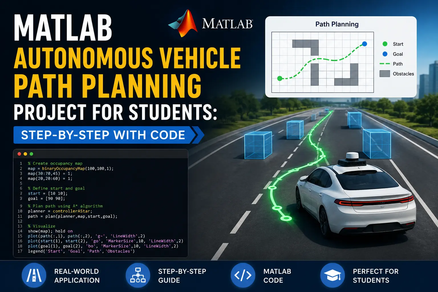
One of the most fascinating and sought-after projects for engineering students is autonomous vehicles. One of the main challenges in the development of self-driving cars is path planning, which is the process of determining a safe, collision-free route from start to objective while taking vehicle restrictions into account. 

This beginner-to-intermediate tutorial will teach you how to use MATLAB and Simulink to create global path planning (using A* or RRT) along with trajectory tracking (e.g., Pure Pursuit or MPC). This project is appropriate for final-year, capstone, or thesis work in the fields of robotics, mechanical, electrical, or mechatronics.

Why Students Love This Project: 

• Integrates modeling, algorithms, simulation, and visualization.
• Very amazing and searchable on GitHub and resumes.
• Makes use of industry-standard tools (MPC Toolbox, Automated Driving Toolbox, and Navigation Toolbox).
• Easy to expand (hardware, dynamic environments, barriers).

MATLAB, Simulink, Navigation Toolbox (for planning), and maybe Model Predictive Control Toolbox are prerequisites.

Step 1: Set Up the Environment and Map

% Load or create occupancy map
load('exampleMap.mat', 'map');  % Or create one
occMap = occupancyMap(map, 10);  % Resolution example

% Inflate obstacles for safety margin
inflatedMap = copy(occMap);
inflate(inflatedMap, 0.5);  % meters

show(inflatedMap);

startPose = [-1, 0, pi/2];
goalPose  = [10, -2, 0];

% State space and planner
ss = stateSpaceSE2;  % or Dubins for vehicles
ss.StateBounds = [inflatedMap.XWorldLimits; inflatedMap.YWorldLimits; [-pi pi]];

stateValidator = validatorOccupancyMap(ss);
stateValidator.Map = inflatedMap;
stateValidator.ValidationDistance = 0.1;

planner = plannerAStarGrid(inflatedMap);  % Simple grid version
% Or Hybrid A* for non-holonomic vehicles: plannerHybridAStar

ss = stateSpaceDubins(bounds);
ss.MinTurningRadius = 0.5;  % Vehicle constraint

stateValidator = validatorOccupancyMap(ss);
stateValidator.Map = inflatedMap;

planner = plannerRRT(ss, stateValidator);
planner.MaxConnectionDistance = 2;
planner.MaxIterations = 10000;

rng default;
[pathObj, solnInfo] = plan(planner, startPose, goalPose);

shortenedPath = shortenpath(pathObj, stateValidator);

show(occMap);
hold on;
plot(pathObj.States(:,1), pathObj.States(:,2), 'r-', 'LineWidth', 2);
plot(shortenedPath.States(:,1), shortenedPath.States(:,2), 'g-', 'LineWidth', 3);

% Simple discrete update (or use Simulink Bicycle Model block)
function [xNext] = bicycleKinematics(x, u, dt)
    xNext = zeros(3,1);
    v = u(1);      % speed
    delta = u(2);  % steering
    L = 2.5;       % wheelbase
    xNext(1) = x(1) + v * cos(x(3)) * dt;
    xNext(2) = x(2) + v * sin(x(3)) * dt;
    xNext(3) = x(3) + (v / L) * tan(delta) * dt;
end

x = startPose';
dt = 0.1;
for i = 1:500
    [v, delta] = controller(x(1:2));   % or MPC output
    u = [v; delta];
    x = bicycleKinematics(x, u, dt);
    
    % Check distance to goal, collision, etc.
    plot(x(1), x(2), 'bo');
    pause(0.01);
end