Reinforcement Learning for Microgrid Energy Management in MATLAB & Simulink

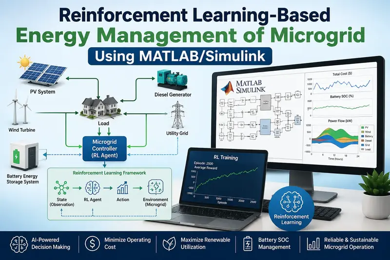
Operating a modern microgrid is an ongoing balancing act. Between changing solar output, shifting wind speeds, volatile electricity pricing, and unpredictable consumer demand, an Energy Management System (EMS) must make real-time decisions every few seconds. It must decide whether to draw electricity from the main grid, fire up a backup generator, or cycle the battery bank, all while protecting sensitive equipment from excessive wear.

The Problem with Traditional Control

Most microgrids in operation today rely on two conventional control methods, both of which run into limitations under high renewable penetration:

• Rule-Based Logic (State Machines): Predefined rules (such as charging the battery whenever surplus solar is available) are simple to build in Stateflow, but they cannot adapt to changing hourly tariffs or plan ahead for upcoming weather shifts.
• Model Predictive Control (MPC): MPC uses numerical optimization across a rolling forecast window. While effective, it requires precise mathematical models of every electrical component, demands significant computing power, and struggles whenever real conditions deviate from forecasts.

Deep Reinforcement Learning (RL) removes this computational bottleneck. Because the complex optimization is performed offline during the training phase, the finished neural network can make dispatch decisions in less than a millisecond on standard embedded controllers.

Structuring the Microgrid as an RL Problem

To train an agent in MATLAB, the microgrid dispatch task is framed as a Markov Decision Process (MDP) with three core elements:

1. Observation Space (What the Agent Sees)

At each control step, the policy receives a continuous sensor vector containing:

• Battery State of Charge (SoC), maintained within a 10% to 90% measurable range.
• Combined renewable generation from solar panels and wind turbines (in kW).
• Total electrical load demand from critical and non-critical circuits (in kW).
• Current electricity tariff rate (in dollars per kWh).
• Time indicators (hour of the day and day of the week) to capture recurring daily demand patterns.

2. Action Space (What the Agent Controls)

Because power converter setpoints require smooth, continuous adjustments rather than discrete switches, continuous-action algorithms such as TD3 (Twin Delayed DDPG) or SAC (Soft Actor-Critic) are used. The policy outputs normalized values between -1.0 and +1.0:

• Battery Power Command: Ranging from maximum charge rate (-P_ch,max) to maximum discharge rate (+P_dis,max).
• Generator Output: Throttling the backup generator from 0 to its maximum rated capacity.
• Grid Power: Acts as the automatic slack balance to absorb remaining energy surpluses or supply deficits.

3. Reward Function Design

The reward function translates operational goals into scalar feedback. At each simulation step, the total reward combines financial costs and operational safety penalties:

Reward = - [ (w₁ × Grid Cost) + (w₂ × Fuel Cost) + (w₃ × Battery Degradation Penalty) + (w₄ × Voltage Penalty) ]

• Grid Cost: The direct price of importing power during peak tariff windows, balanced against revenue earned from exporting clean power back to the grid.
• Fuel Cost: The fuel consumption expense of running diesel or gas generators.
• Battery Degradation Penalty: A quadratic penalty applied whenever the battery State of Charge drifts outside the optimal 20% to 80% operating window, as well as penalties for aggressive high-current cycling.
• Voltage Penalty: A strict penalty applied if the local AC bus voltage deviates beyond standard utility limits (plus or minus 5%).

Implementation Workflow in MATLAB and Simulink

MATLAB and Simulink allow complete co-simulation between physical electrical models and learning agents:

1. Build the Physical Microgrid in Simscape Electrical: Model your solar array, battery bank, inverters, and electrical loads using Simscape physical blocks. Using a discrete solver with a sample time between 0.1 and 1.0 second keeps simulation runtimes manageable during long training runs.
2. Embed the RL Agent Block: Place the Reinforcement Learning Agent block from the Reinforcement Learning Toolbox directly into your Simulink harness to link sensor signals to the policy.
3. Add a Safety Clamping Layer: Never route raw neural network outputs directly into physical converters. Always insert a deterministic saturation block between the agent and converter gate drivers to enforce hard voltage, current, and thermal limits during initial exploration.
4. Apply Domain Randomization: At the start of each training episode, randomize starting battery charge levels (between 30% and 80%), solar irradiance profiles, and load curves to prevent the policy from overfitting to a single operational day.

Practical Tips for Stable Training

• Break Algebraic Loops: When connecting the RL block to electrical circuits in Simulink, place a Unit Delay block on the feedback signals. This eliminates algebraic loop warnings and substantially accelerates solver speeds.
• Normalize Sensor Inputs: Scale all observation inputs to roughly the -1.0 to +1.0 range before feeding them into the actor and critic networks to keep gradient updates stable.
• Code Generation: After training reaches steady reward convergence, you can export the trained actor policy to C or C++ code using MATLAB Coder for deployment on industrial microgrid PLCs.