Estimate the Transfer Function of an Unknown System

You can estimate the transfer function of an unknown system based on the system's measured input and output data.

In DSP System Toolbox™, you can estimate the transfer function of a system using the dsp.TransferFunctionEstimator System object™ in MATLAB^® and the Discrete Transfer Function Estimator block in Simulink^®. The relationship between the input x and output y is modeled by the linear, time-invariant transfer function T_xy. The transfer function is the ratio of the cross power spectral density of x and y, P_yx, to the power spectral density of x, P_xx:

Txy(f)=Pyx(f)Pxx(f)

The dsp.TransferFunctionEstimator object and Discrete Transfer Function Estimator block use the Welch’s averaged periodogram method to compute the P_xx and P_xy. For more details on this method, see Spectral Analysis.

Coherence

The coherence, or magnitude-squared coherence, between x and y is defined as:

Cxy(f)=?Pxy?2Pxx∗Pyy

The coherence function estimates the extent to which you can predict y from x. The value of the coherence is in the range 0 ≤ C_xy(f) ≤ 1. If C_xy = 0, the input x and output y are unrelated. A C_xy value greater than 0 and less than 1 indicates one of the following:

Measurements are noisy.
The system is nonlinear.
Output y is a function of x and other inputs.

The coherence of a linear system represents the fractional part of the output signal power that is produced by the input at that frequency. For a particular frequency, 1 – C_xy is an estimate of the fractional power of the output that the input does not contribute to.

When you set the OutputCoherence property of dsp.TransferFunctionEstimator to true, the object computes the output coherence. In the Discrete Transfer Function Estimator block, to compute the coherence spectrum, select the Output magnitude squared coherence estimate check box.

Estimate the Transfer Function in MATLAB

To estimate the transfer function of a system in MATLAB™, use the dsp.TransferFunctionEstimator System object™. The object implements the Welch's average modified periodogram method and uses the measured input and output data for estimation.

Initialize the System

The system is a cascade of two filter stages: dsp.LowpassFilter and a parallel connection of dsp.AllpassFilter and dsp.AllpoleFilter.

allpole = dsp.AllpoleFilter;
allpass = dsp.AllpassFilter;
lpfilter = dsp.LowpassFilter;

Specify Signal Source

The input to the system is a sine wave with a frequency of 100 Hz. The sampling frequency is 44.1 kHz.

sine = dsp.SineWave('Frequency',100,'SampleRate',44100,...
    'SamplesPerFrame',1024);

Create Transfer Function Estimator

To estimate the transfer function of the system, create the dsp.TransferFunctionEstimator System object.

tfe  = dsp.TransferFunctionEstimator('FrequencyRange','onesided',...
    'OutputCoherence', true);

Create Array Plot

Initialize two dsp.ArrayPlot objects: one to display the magnitude response of the system and the other to display the coherence estimate between the input and the output.

tfeplotter = dsp.ArrayPlot('PlotType','Line',...
    'XLabel','Frequency (Hz)',...
    'YLabel','Magnitude Response (dB)',...
    'YLimits',[-120 20],...
    'XOffset',0,...
    'XLabel','Frequency (Hz)',...
    'Title','System Transfer Function',...
    'SampleIncrement',44100/1024);
coherenceplotter = dsp.ArrayPlot('PlotType','Line',...
    'YLimits',[0 1.2],...
    'YLabel','Coherence',...
    'XOffset',0,...
    'XLabel','Frequency (Hz)',...
    'Title','Coherence Estimate',...
    'SampleIncrement',44100/1024);

By default, the x-axis of the array plot is in samples. To convert this axis into frequency, set the 'SampleIncrement' property of the dsp.ArrayPlot object to Fs/1024. In this example, this value is 44100/1024, or 43.0664. For a two-sided spectrum, the XOffset property of the dsp.ArrayPlot object must be [-Fs/2]. The frequency varies in the range [-Fs/2 Fs/2]. In this example, the array plot shows a one-sided spectrum. Hence, set the XOffset to 0. The frequency varies in the range [0 Fs/2].

Estimate the Transfer Function

The transfer function estimator accepts two signals: input to the two-stage filter and output of the two-stage filter. The input to the filter is a sine wave containing additive white Gaussian noise. The noise has a mean of zero and a standard deviation of 0.1. The estimator estimates the transfer function of the two-stage filter. The output of the estimator is the frequency response of the filter, which is complex. To extract the magnitude portion of this complex estimate, use the abs function. To convert the result into dB, apply a conversion factor of 20*log10(magnitude).

for Iter = 1:1000
    input = sine() + .1*randn(1024,1);
    lpfout = lpfilter(input);
    allpoleout = allpole(lpfout);
    allpassout = allpass(lpfout);
    output = allpoleout + allpassout;
    [tfeoutput,outputcoh] = tfe(input,output);
    tfeplotter(20*log10(abs(tfeoutput)));
    coherenceplotter(outputcoh);
end

The first plot shows the magnitude response of the system. The second plot shows the coherence estimate between the input and output of the system. Coherence in the plot varies in the range [0 1] as expected.

Magnitude Response of the Filter Using fvtool

The filter is a cascade of two filter stages - dsp.LowpassFilter and a parallel connection of dsp.AllpassFilter and dsp.AllpoleFilter. All the filter objects are used in their default state. Using the filter coefficients, derive the system transfer function and plot the frequency response using freqz. Below are the coefficients in the [Num] [Den] format:

All pole filter - [1 0] [1 0.1]
All pass filter - [0.5 -1/sqrt(2) 1] [1 -1/sqrt(2) 0.5]
Lowpass filter - Determine the coefficients using the following commands:

lpf = dsp.LowpassFilter;
Coefficients = coeffs(lpf);

Coefficients.Numerator gives the coefficients in an array format. The mathematical derivation of the overall system transfer function is not shown here. Once you derive the transfer function, run fvtool and you can see the frequency response below:

The magnitude response that fvtool shows matches the magnitude response that the dsp.TransferFunctionEstimator object estimates.

Estimate the Transfer Function in Simulink

To estimate the transfer function of a system in Simulink, use the Discrete Transfer Function Estimator block. The block implements the Welch's average modified periodogram method and uses the measured input and output data for estimation.

The system is a cascade of two filter stages: a lowpass filter and a parallel connection of an allpole filter and allpass filter. The input to the system is a sine wave containing additive white Gaussian noise. The noise has a mean of zero and a standard deviation of 0.1. The input to the estimator is the system input and the system output. The output of the estimator is the frequency response of the system, which is complex. To extract the magnitude portion of this complex estimate, use the Abs block. To convert the result into dB, the system uses a dB (1 ohm) block.

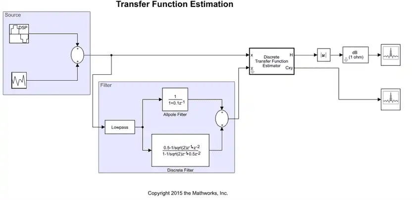
Snapshot of the transfer function estimator model. Source blocks on the left followed by the filter cascade blocks, transfer function estimator, Abs block, dB Conversion block, and two Array Plot blocks.

Open and Inspect the Model

To open the model, enter ex_transfer_function_estimator in the MATLAB command prompt.

Here are the settings of the blocks in the model.

Block	Parameter Changes	Purpose of the block
Sine Wave	Sample time to `1/44100` Samples per frame to `1024`	Sinusoid signal with frequency at 100 Hz
Random Source	Source type to `Gaussian` Variance to 0.01 Sample time to 1/44100 Samples per frame to 1024	Random Source block generates a random noise signal with properties specified through the block dialog box
Lowpass Filter	No change	Lowpass filter
Allpole Filter	No change	Allpole filter with coefficients `[1 0.1]`
Discrete Filter	Numerator to `[0.5 -1/sqrt(2) 1]` Denominator to `[1 -1/sqrt(2) 0.5]`	Allpass filter with coefficients `[-1/sqrt(2) 0.5]`
Discrete Transfer Function Estimator	Frequency range to `One-sided` Number of spectral averages to 8	Transfer function estimator
Abs	No change	Extracts the magnitude information from the output of the transfer function estimator
First Array Plot block	Click View: Select Style and set Plot type to `Line`. Select Configuration Properties: From the Main tab, set Sample increment to `44100/1024` and X-offset to `0`. In the Display tab, specify the Title as `Magnitude Response of the System in dB`, X-label as `Frequency (Hz)`, and Y-label as `Amplitude (dB)`	Shows the magnitude response of the system
Second Array Plot block	Click View: Select Style and set Plot type to `Line`. Select Configuration Properties: From the Main tab, set Sample increment to `44100/1024` and X-offset to `0`. In the Display tab, specify the Title as `Coherence Estimate`, X-label as `Frequency (Hz)`, and Y-label as `Amplitude`	Shows the coherence estimate

By default, the x-axis of the array plot is in samples. To convert this axis into frequency, the Sample increment parameter is set to Fs/1024. In this example, this value is 44100/1024, or 43.0664. For a two-sided spectrum, the X-offset parameter must be –Fs/2. The frequency varies in the range [-Fs/2 Fs/2]. In this example, the array plot shows a one-sided spectrum. Hence, the X-offset is set to 0. The frequency varies in the range [0 Fs/2].

Run the Model

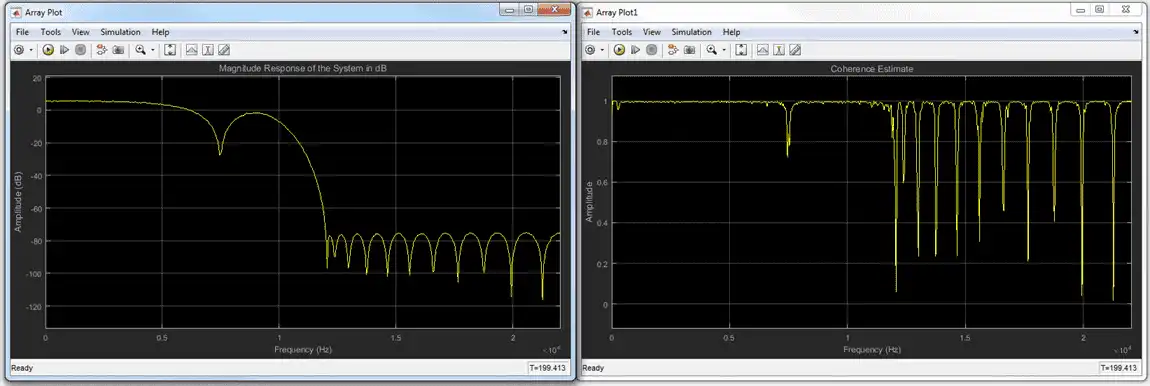
Output of the two Array Plot blocks are placed next to each other. First Array Plot block on the left shows the magnitude response of the system in dB. The second Array Plot block on the right shows the coherence estimate. The x-axis for both plots shows the frequencies in Hz, ranging from 0 to 22500 Hz.

Matlabsolutions.com provides guaranteed satisfaction with a commitment to complete the work within time. Combined with our meticulous work ethics and extensive domain experience, We are the ideal partner for all your homework/assignment needs. We pledge to provide 24*7 support to dissolve all your academic doubts. We are composed of 300+ esteemed Matlab and other experts who have been empanelled after extensive research and quality check.

Matlabsolutions.com provides undivided attention to each Matlab assignment order with a methodical approach to solution. Our network span is not restricted to US, UK and Australia rather extends to countries like Singapore, Canada and UAE. Our Matlab assignment help services include Image Processing Assignments, Electrical Engineering Assignments, Matlab homework help, Matlab Research Paper help, Matlab Simulink help. Get your work done at the best price in industry.