Estimate the Power Spectrum in MATLAB

The power spectrum (PS) of a time-domain signal is the distribution of power contained within the signal over frequency, based on a finite set of data. The frequency-domain representation of the signal is often easier to analyze than the time-domain representation. Many signal processing applications, such as noise cancellation and system identification, are based on the frequency-specific modifications of signals. The goal of the power spectral estimation is to estimate the power spectrum of a signal from a sequence of time samples. Depending on what is known about the signal, estimation techniques can involve parametric or nonparametric approaches and can be based on time-domain or frequency-domain analysis. For example, a common parametric technique involves fitting the observations to an autoregressive model. A common nonparametric technique is the periodogram. The power spectrum is estimated using Fourier transform methods such as the Welch method and the filter bank method. For signals with relatively small length, the filter bank approach produces a spectral estimate with a higher resolution, a more accurate noise floor, and peaks more precise than the Welch method, with low or no spectral leakage. These advantages come at the expense of increased computation and slower tracking. For more details on these methods, see Spectral Analysis. You can also use other techniques such as the maximum entropy method.

In MATLAB^®, you can perform real-time spectral analysis of a dynamic signal using the dsp.SpectrumAnalyzer System object™. You can view the spectral data in the spectrum analyzer and store the data in a workspace variable using the isNewDataReady and getSpectrumData object functions. Alternately, you can use the dsp.SpectrumEstimator System object followed by dsp.ArrayPlot object to view the spectral data. The output of the dsp.SpectrumEstimator object is the spectral data. This data can be acquired for further processing.

Estimate the Power Spectrum Using dsp.SpectrumAnalyzer

To view the power spectrum of a signal, you can use the dsp.SpectrumAnalyzer System object™. You can change the dynamics of the input signal and see the effect those changes have on the power spectrum of the signal in real time.

Initialization

Initialize the sine wave source to generate the sine wave and the spectrum analyzer to show the power spectrum of the signal. The input sine wave has two frequencies: one at 1000 Hz and the other at 5000 Hz. Create two dsp.SineWave objects, one to generate the 1000 Hz sine wave and the other to generate the 5000 Hz sine wave.

Fs = 44100;
Sineobject1 = dsp.SineWave('SamplesPerFrame',1024,'PhaseOffset',10,...
    'SampleRate',Fs,'Frequency',1000);
Sineobject2 = dsp.SineWave('SamplesPerFrame',1024,...
    'SampleRate',Fs,'Frequency',5000);
SA = dsp.SpectrumAnalyzer('SampleRate',Fs,'Method','Filter bank',...
    'SpectrumType','Power','PlotAsTwoSidedSpectrum',false,...
    'ChannelNames',{'Power spectrum of the input'},'YLimits',[-120 40],'ShowLegend',true);

The spectrum analyzer uses the filter bank approach to compute the power spectrum of the signal.

Estimation

Stream in and estimate the power spectrum of the signal. Construct a for-loop to run for 5000 iterations. In each iteration, stream in 1024 samples (one frame) of each sine wave and compute the power spectrum of each frame. To generate the input signal, add the two sine waves. The resultant signal is a sine wave with two frequencies: one at 1000 Hz and the other at 5000 Hz. Add Gaussian noise with zero mean and a standard deviation of 0.001. To acquire the spectral data for further processing, use the isNewDataReady and the getSpectrumData object functions. The variable data contains the spectral data that is displayed on the spectrum analyzer along with additional statistics about the spectrum.

data = [];
for Iter = 1:7000
    Sinewave1 = Sineobject1();
    Sinewave2 = Sineobject2();
    Input = Sinewave1 + Sinewave2;
    NoisyInput = Input + 0.001*randn(1024,1);
    SA(NoisyInput);
     if SA.isNewDataReady
        data = [data;getSpectrumData(SA)];
     end
end
release(SA);

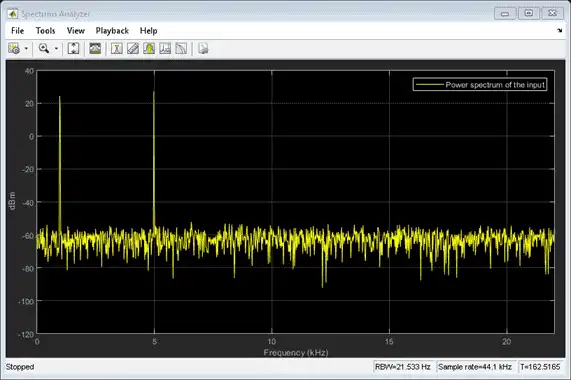
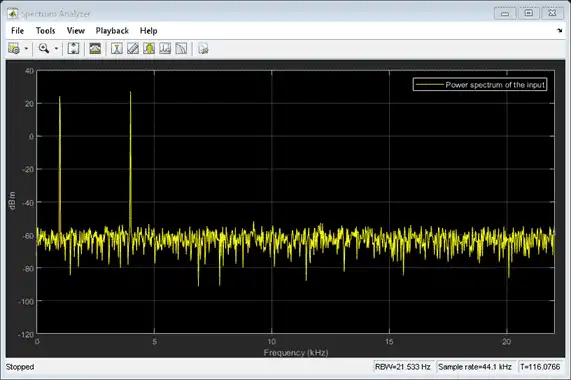
In the spectrum analyzer output, you can see two distinct peaks: one at 1000 Hz and the other at 5000 Hz.

Resolution Bandwidth (RBW) is the minimum frequency bandwidth that can be resolved by the spectrum analyzer. By default, the RBWSource property of the dsp.SpectrumAnalyzer object is set to Auto. In this mode, RBW is the ratio of the frequency span to 1024. In a two-sided spectrum, this value is $\frac{F_{s}}{1024}$ , while in a one-sided spectrum, it is $\frac{\frac{F_{s}}{2}}{1024}$ . The spectrum analyzer in this example shows a one-sided spectrum. Hence, RBW is (44100/2)/1024 or 21.53Hz

Using this value of $RBW$ , the number of input samples required to compute one spectral update, $N_{samples}$ is given by the following equation: $N_{samples} = \frac{F_{s}}{RBW}$ .

In this example, $N_{samples}$ is 44100/21.53 or 2048 samples.

$RBW$ calculated in the 'Auto' mode gives a good frequency resolution.

To distinguish between two frequencies in the display, the distance between the two frequencies must be at least RBW. In this example, the distance between the two peaks is 4000 Hz, which is greater than $RBW$ . Hence, you can see the peaks distinctly. Change the frequency of the second sine wave to 1015 Hz. The difference between the two frequencies is less than $RBW$ .

release(Sineobject2);
Sineobject2.Frequency = 1015;
for Iter = 1:5000
    Sinewave1 = Sineobject1();
    Sinewave2 = Sineobject2();
    Input = Sinewave1 + Sinewave2;
    NoisyInput = Input + 0.001*randn(1024,1);
    SA(NoisyInput);
end
release(SA);

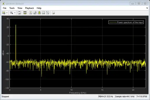
The peaks are not distinguishable.

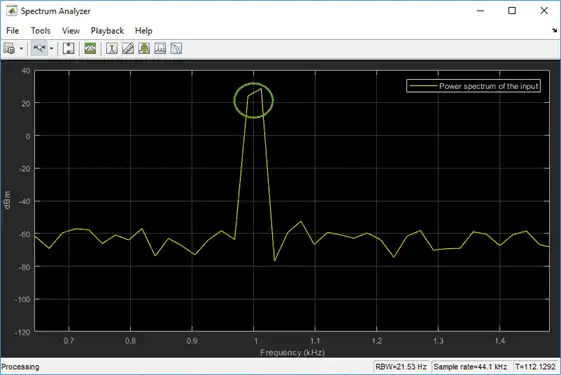
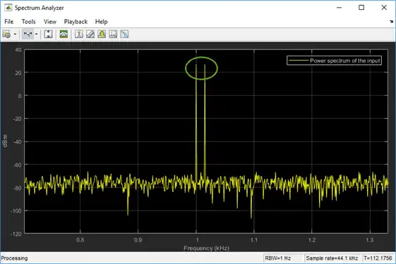
To increase the frequency resolution, decrease $RBW$ to 1 Hz.

SA.RBWSource = 'property';
SA.RBW = 1;
for Iter = 1:5000
    Sinewave1 = Sineobject1();
    Sinewave2 = Sineobject2();
    Input = Sinewave1 + Sinewave2;
    NoisyInput = Input + 0.001*randn(1024,1);
    SA(NoisyInput);
end
release(SA);

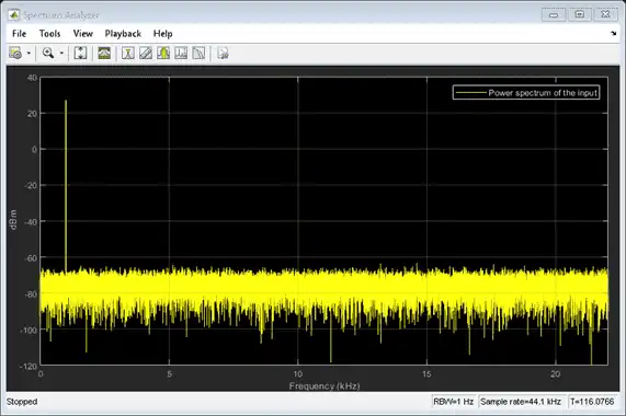
On zooming, the two peaks, which are 15 Hz apart, are now distinguishable.

When you increase the frequency resolution, the time resolution decreases. To maintain a good balance between the frequency resolution and time resolution, change the RBWSource property to Auto.

During streaming, you can change the input properties or the spectrum analyzer properties and see the effect on the spectrum analyzer output immediately. For example, change the frequency of the second sine wave when the index of the loop is a multiple of 1000.

release(Sineobject2);
SA.RBWSource = 'Auto';
for Iter = 1:5000
    Sinewave1 = Sineobject1();
    if (mod(Iter,1000) == 0)
        release(Sineobject2);
        Sineobject2.Frequency = Iter;
        Sinewave2 = Sineobject2();
    else
        Sinewave2 = Sineobject2();
    end
    Input = Sinewave1 + Sinewave2;
    NoisyInput = Input + 0.001*randn(1024,1);
    SA(NoisyInput);
end
release(SA);

While running the streaming loop, you can see that the peak of the second sine wave changes according to the iteration value. Similarly, you can change any of the spectrum analyzer properties while the simulation is running and see a corresponding change in the output.

Convert the Power Between Units

The spectrum analyzer provides three units to specify the power spectral density: Watts/Hz, dBm/Hz, and dBW/Hz. Corresponding units of power are Watts, dBm, and dBW. For electrical engineering applications, you can also view the RMS of your signal in Vrms or dBV. The default spectrum type is Power in dBm.

Convert the Power in Watts to dBW and dBm

Power in dBW is given by:

PdBW=10log10(power in watt/1 watt)

Power in dBm is given by:

PdBm=10log10(power in watt/1 milliwatt)

For a sine wave signal with an amplitude of 1 V, the power of a one-sided spectrum in Watts is given by:

PWatts=A2/2PWatts=1/2

In this example, this power equals 0.5 W. Corresponding power in dBm is given by:

PdBm=10log10(power in watt/1 milliwatt)PdBm=10log10(0.5/10−3)

Here, the power equals 26.9897 dBm. To confirm this value with a peak finder, click Tools > Measurements > Peak Finder.

For a white noise signal, the spectrum is flat for all frequencies. The spectrum analyzer in this example shows a one-sided spectrum in the range [0 Fs/2]. For a white noise signal with a variance of 1e-4, the power per unit bandwidth (P_{unitbandwidth}) is 1e-4. The total power of white noise in watts over the entire frequency range is given by:

Pwhitenoise=Punitbandwidth∗number of frequency bins,Pwhitenoise=(10−4)∗(Fs/2RBW),Pwhitenoise=(10−4)∗(2205021.53)

The number of frequency bins is the ratio of total bandwidth to RBW. For a one-sided spectrum, the total bandwidth is half the sampling rate. RBW in this example is 21.53 Hz. With these values, the total power of white noise in watts is 0.1024 W. In dBm, the power of white noise can be calculated using 10*log10(0.1024/10^-3), which equals 20.103 dBm.

Convert Power in Watts to dBFS

If you set the spectral units to dBFS and set the full scale (FullScaleSource) to Auto, power in dBFS is computed as:

PdBFS=20⋅log10(√Pwatts/Full_Scale)

where:

P_watts is the power in watts
For double and float signals, Full_Scale is the maximum value of the input signal.
For fixed point or integer signals, Full_Scale is the maximum value that can be represented.

If you specify a manual full scale (set FullScaleSource to Property), power in dBFS is given by:

PFS=20⋅log10(√Pwatts/FS)

Where FS is the full scaling factor specified in the FullScale property.

For a sine wave signal with an amplitude of 1 V, the power of a one-sided spectrum in Watts is given by:

PWatts=A2/2PWatts=1/2

In this example, this power equals 0.5 W and the maximum input signal for a sine wave is 1 V. The corresponding power in dBFS is given by:

PFS=20⋅log10(√1/2/1)

Here, the power equals -3.0103. To confirm this value in the spectrum analyzer, run these commands:

Fs = 1000;  % Sampling frequency
sinef = dsp.SineWave('SampleRate',Fs,'SamplesPerFrame',100);
scope = dsp.SpectrumAnalyzer('SampleRate',Fs,...
   'SpectrumUnits','dBFS','PlotAsTwoSidedSpectrum',false)
%%
for ii = 1:100000
xsine = sinef();
scope(xsine)
end

Then, click Tools > Measurements > Peak Finder.

Convert the Power in dBm to RMS in Vrms

Power in dBm is given by:

PdBm=10log10(power in watt/1 milliwatt)

Voltage in RMS is given by:

Vrms=10PdBm/20√10−3

From the previous example, P_dBm equals 26.9897 dBm. The V_rms is calculated as

Vrms=1026.9897/20√0.001

which equals 0.7071.

To confirm this value:

Change Type to RMS.
Open the peak finder by clicking Tools > Measurements > Peak Finder.

Estimate the Power Spectrum Using dsp.SpectrumEstimator

Alternately, you can compute the power spectrum of the signal using the dsp.SpectrumEstimator System object. You can acquire the output of the spectrum estimator and store the data for further processing. To view other objects in the Estimation library, type help dsp in the MATLAB® command prompt, and click Estimation.

Initialization

Use the same source as in the previous section on using the dsp.SpectrumAnalyzer to estimate the power spectrum. The input sine wave has two frequencies: one at 1000 Hz and the other at 5000 Hz. Initialize dsp.SpectrumEstimator to compute the power spectrum of the signal using the filter bank approach. View the power spectrum of the signal using the dsp.ArrayPlot object.

Fs = 44100;
Sineobject1 = dsp.SineWave('SamplesPerFrame',1024,'PhaseOffset',10,...
    'SampleRate',Fs,'Frequency',1000);
Sineobject2 = dsp.SineWave('SamplesPerFrame',1024,...
    'SampleRate',Fs,'Frequency',5000);

SpecEst = dsp.SpectrumEstimator('Method','Filter bank',...
    'PowerUnits','dBm','SampleRate',Fs,'FrequencyRange','onesided');
ArrPlot = dsp.ArrayPlot('PlotType','Line','ChannelNames',{'Power spectrum of the input'},...
    'YLimits',[-80 30],'XLabel','Number of samples per frame','YLabel',...
    'Power (dBm)','Title','One-sided power spectrum with respect to samples');

Matlabsolutions.com provides guaranteed satisfaction with a commitment to complete the work within time. Combined with our meticulous work ethics and extensive domain experience, We are the ideal partner for all your homework/assignment needs. We pledge to provide 24*7 support to dissolve all your academic doubts. We are composed of 300+ esteemed Matlab and other experts who have been empanelled after extensive research and quality check.

Matlabsolutions.com provides undivided attention to each Matlab assignment order with a methodical approach to solution. Our network span is not restricted to US, UK and Australia rather extends to countries like Singapore, Canada and UAE. Our Matlab assignment help services include Image Processing Assignments, Electrical Engineering Assignments, Matlab homework help, Matlab Research Paper help, Matlab Simulink help. Get your work done at the best price in industry.