Design of Decimators and Interpolators

this example shows how to design filters for decimation and interpolation of discrete sequences.

The Role of Lowpass Filtering in Rate Conversion

Rate conversion is the process of changing the rate of a discrete signal to obtain a new discrete representation of the underlying continuous signal. The process involves uniform downsampling and upsampling. Uniform downsampling by a rate of N refers to taking every N-th sample of a sequence and discarding the rest of the samples. Uniform upsampling by a factor of N refers to the padding of N-1 zeros between every two consecutive samples.

x = 1:3
L = 3; % upsampling rate
M = 2; % downsampling rate

% Upsample and downsample
xUp = upsample(x,L)
xDown = downsample(x,M)

x =

     1     2     3


xUp =

     1     0     0     2     0     0     3     0     0


xDown =

     1     3

Both those basic operations introduce signal artifacts: downsampling introduces aliasing, and upsampling introduces imaging. To mitigate these effect, use lowpass filters.

When downsampling by a rate of , a lowpass filter applied prior to downsampling limits the input bandwidth, and thus eliminating spectrum aliasing. This is similar to an analog LPF used in A/D converters. Ideally, such an anti-aliasing filter has a unit gain and a cutoff frequency of $\omega_c = \frac{1}{N}\omega_N$ , here $\omega_N$ is the Nyquist frequency of the signal. Note: the underlying sampling frequency is insignificant, we assume normalized frequencies (i.e. $\omega_N=1$ ) throughout the discussion.
When upsampling by a rate of , a lowpass filter applied after upsampling is known as an anti-imaging filter. The filter removes the spectral images of the low-rate signal. Ideally, the cutoff frequency of this anti-imaging filter is $\omega_c = \frac{1}{N}$ (like its antialiasing counterpart), while its gain is .

Both upsampling and downsampling operations of rate $N$ require a lowpass filter with a normalized cutoff frequency of $\frac{1}{N}$ . The only difference is in the required gain and the placement of the filter (before or after rate conversion).

The combination of upsampling a signal by a factor of $L$ , followed by filtering, and then downsampling by a factor of $M$ converts the sequence sample rate by a rational factor of $\frac{L}{M}$ . This is obtained by upsampling by rate $L$ followed by filtering, then downsampling by rate $M$ . The order of rate conversion operation cannot be commuted. A single filter that combines anti-aliasing and anti-imaging is placed between the upsampling and the downsampling stages. This filter is a lowpass with the normalized cutoff frequency of $\omega_c=\min(1/L,1/M)$ and a gain of $L$ .

While any lowpass FIR design function (e.g. fir1, firpm, or fdesign) could design an appropriate anti-aliasing and anti-imaging filter, the function designMultirateFIR gives a convenient and a simplified interface. The next few sections show the use of these functions to design the filter and demonstrate why designMultirateFIR is the preferred way.

Filtered Rate Conversion: Decimators, Interpolators, and Rational Rate Converters

Filtered rate conversions includes decimators, interpolators, and rational rate converters, all of which are cascades of rate change blocks with filters in various configuations.

Filtered Rate Conversion using the filter, upsample, and downsample functions

Decimation refers to LTI filtering followed by uniform downsampling. An FIR decimator can be implemented as follows.

Design a an anti-aliasing lowpass filter h
Filter the input though h
Downsample the filtered sequence by a factor of M

% Define an input sequence
x = rand(60,1);

% Implement an FIR decimator
h = fir1(L*12*2,1/M); % an arbitrary filter
xDecim = downsample(filter(h,1,x), M);

Interpolation refers to a upsampling followed by filtering. The implementation is very similar to decimation.

xInterp = filter(h,1,upsample(x,L));

Lastly, rational rate conversion is comprised of an interpolator followed by a decimator (in that specific order).

xRC = downsample(filter(h,1,upsample(x,L) ), M);

Filtered Rate Conversion Using System Objects

For streaming data, the system objects dsp.FIRInterpolator, dsp.FIRDecimator, and dsp.FIRRateConverter encapsulate the rate change and filtering in a single object. For example, construction of an interpolator is done as follows.

firInterp = dsp.FIRInterpolator(L,h);

Then, feed a sequence to the newly created object by a step call.

xInterp = firInterp(x);

Design and use decimators and rate converters in a similar way.

firDecim = dsp.FIRDecimator(M,h); % Construct
xDecim = firDecim(x); % Decimate (step call)

firRC = dsp.FIRRateConverter(L,M,h); % Construct
xRC = firRC(x); % Convert rate (step call)

Using system objects is generally preferred, as they:

Allow for a cleaner syntax.
Keep a state, as filter initial coniditon for subsequent step calls.
Most importantly, they utilize a very efficient polyphase algorithm.

To construct these object, you need the rate conversion factor, and the FIR coefficients. The following section describes how to generate appropriate FIR coefficients for a rate conversion filter.

Design a Rate Conversion Filter using `designMultirateFIR`

The function designMultirateFIR(L,M) automatically finds the apropriate scaling and cutoff frequency for a given rate conversion ratio $L/M$ . Use the FIR coefficients returned by designMultirateFIR with dsp.FIRDecimator (if $L=1$ ), dsp.FIRInterpolator (if $M=1$ ), or dsp.FIRRateConverter (general case).

Let us design an interpolation filter:

L = 3;
bInterp = designMultirateFIR(L,1); % Pure upsampling filter
firInterp = dsp.FIRInterpolator(L,bInterp);

Then, apply the interpolator to a sequence.

% Create a sequence
n = (0:89)';
f = @(t) cos(0.1*2*pi*t).*exp(-0.01*(t-25).^2)+0.2;
x = f(n);

% Apply interpolator
xUp = firInterp(x);
release(firInterp);

Let us first examine the raw output of the interpolator and compare with the original sequence.

plot_raw_sequences(x,xUp);

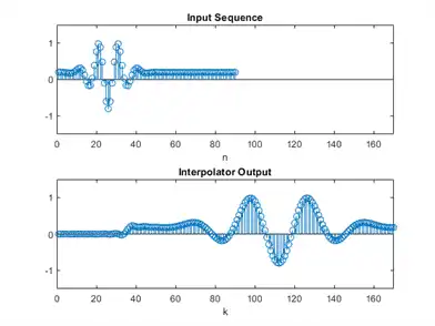
While there is some resemblence between the input x and the output xUp, there are several key differences. In the interpolated signal

The time domain is stretched (as expected).
The signal has a delay of half the length of the FIR length(h)/2 (denoted henceforth).
There is a transient response at the beginning.

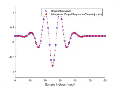
To compare, align and scale the time domains of the two sequences. An interpolated sample xUp[k] corresponds to an input time $t[k]=\frac{1}{L}(k-i_0)$ .

nUp = (0:length(xUp)-1);
i0 = length(bInterp)/2;
plot_scaled_sequences(n,x,(1/L)*(nUp-i0),xUp,["Original Sequence",...
            "Interpolator Output Sequence (Time Adjusted)"],[0,60]);

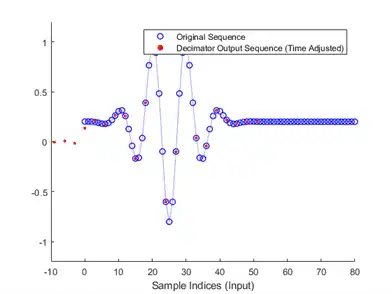
The same idea works for downsampling, where the time conversion is $t[k] = Mk-i_0$ :

M = 3;
bDecim = designMultirateFIR(1,M); % Pure downsampling filter
firDecim = dsp.FIRDecimator(M,bDecim);
xDown = firDecim(x);

Plot them on the same scale and adjust for delay. Note they overlap perfectly.

i0 = length(bDecim)/2;
nDown = (0:length(xDown)-1);
plot_scaled_sequences(n,x,M*nDown-i0,xDown,["Original Sequence",...
            "Decimator Output Sequence (Time Adjusted)"],[-10,80]);

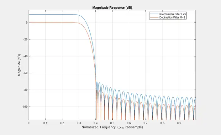
Visualize the magnitude responses of the upsampling and downampling filters using fvtool. The two FIR filters are identical in that case, up to a different gain.

hfv = fvtool(firInterp,firDecim); % Notice the gains in the passband
legend(hfv,"Interpolation Filter L="+num2str(L), ...
            "Decimation Filter M="+num2str(M));

General rational conversions can be treated the same way as upsampling and downsampling. The cutoff is $~\omega_c=\min(\frac{1}{L},~\frac{1}{M})~$ and the gain is $L$ . The function designMultirateFIR figures that out automatically.

L = 5;
M = 2;
b = designMultirateFIR(L,M);
firRC = dsp.FIRRateConverter(L,M,b);

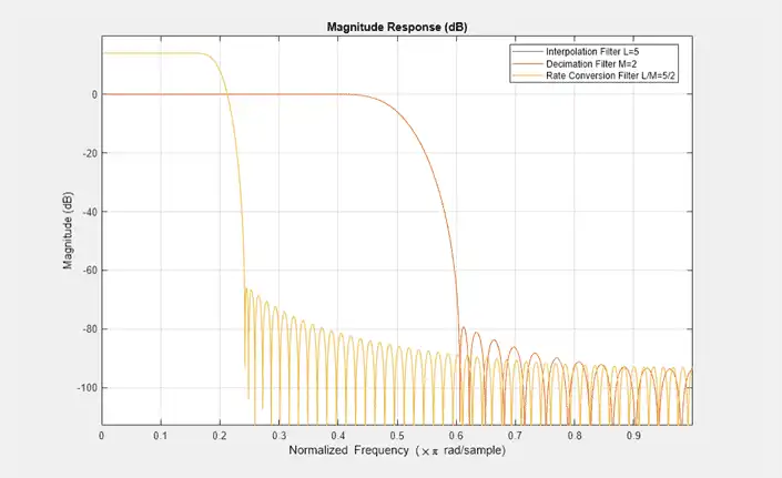
Let us now compare the combined filter with the separate interpolation/decimation components.

firDecim = dsp.FIRDecimator(M,designMultirateFIR(1,M));
firInterp = dsp.FIRInterpolator(L,designMultirateFIR(L,1));

hfv = fvtool(firInterp,firDecim, firRC); % Notice the gains in the passband
legend(hfv,"Interpolation Filter L="+num2str(L),...
    "Decimation Filter M="+num2str(M), ...
    "Rate Conversion Filter L/M="+num2str(L)+"/"+num2str(M));

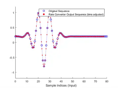
Once the FIRRateConverter is set up, perform the rate conversion by a step call.

xRC = firRC(x);

Plot the input and the filter output with time adjustment given by $t[k] = \frac{1}{L}(Mk-i_0)$ .

nRC = (0:length(xRC)-1)';
i0 = length(b)/2;
plot_scaled_sequences(n,x,(1/L)*(M*nRC-i0),xRC,["Original Sequence",...
        "Rate Converter Output Sequence (time adjusted)"],[0,80]);

Adjusting the Lowpass FIR Design Parameters

Using designMultirateFIR you can also adjust the FIR length, transition width, and stopband attenuation.

Adjusting the FIR Length

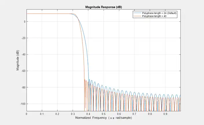
The FIR length can be controlled through L, M, and a third parameter P called half-polyphase length, whose default value is 12 (refer to Output Arguments for more details). Let us examine two design points.

% Unspecified half-length defaults to 12
b24 = designMultirateFIR(3,1);

halfPhaseLength = 20;
b40 = designMultirateFIR(3,1,halfPhaseLength);

Generally, larger half polyphase length yields steeper transitions.

hfv = fvtool(b24,1,b40,1);
legend(hfv, 'Polyphase length = 24 (Default)','Polyphase length = 40');

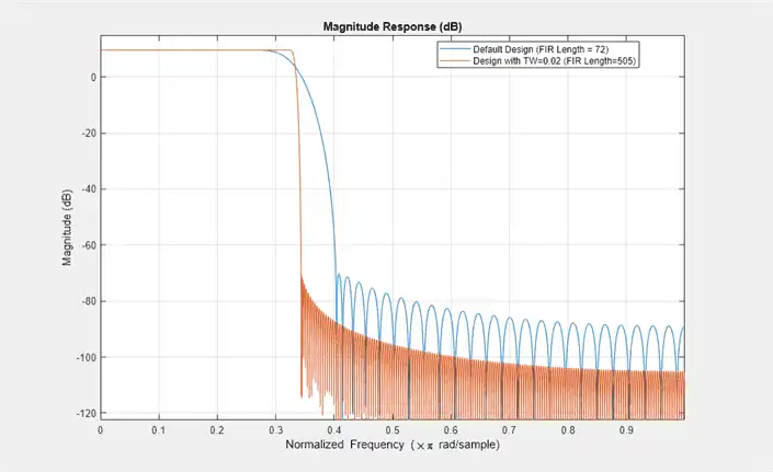
Adjusting the Transition Width

Design the filter by specifying the desired transition width. The appropirate length will be derived automatically. Plot the resulting filter against the default design, and notice the difference in the transition width.

TW = 0.02;
bTW = designMultirateFIR(3,1,TW);

hfv = fvtool(b24,1,bTW,1);
legend(hfv, 'Default Design (FIR Length = 72)',"Design with TW="...
        +num2str(TW)+" (FIR Length="+num2str(length(bTW))+")");

The Special Case of Rate Conversion by 2: Halfband Interpolators and Decimators

Using a half-band filter (i.e. $\omega_c=\frac{1}{2}$ ), you can perform sample rate conversion by a factor of 2. The dsp.FIRHalfbandInterpolator and dsp.FIRHalfbandDecimator objects perform interpolation and decimation by a factor of 2 using halfband filters. These system object are implemented using an efficient polyphase structure specific for that rate conversion. The IIR counterparts dsp.IIRHalfbandInterpolator and dsp.IIRHalfbandDecimator can be even more efficient. These system objects can also work with custom sample rates.

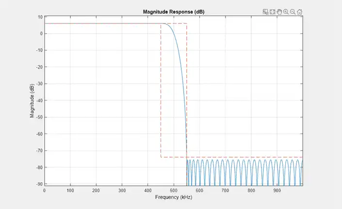
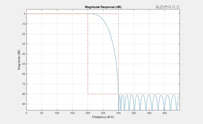
Visualize the magnitude response using fvtool. In the case of interpolation, the filter retains most of the spectrum from 0 to Fs/2 while attenuating spectral images. For decimation, the filter passes about half of the band, that is 0 to Fs/4, and attenuates the other half in order to minimize aliasing. The amount of attenuation can be set to any desired value for both interpolation and decimation. If unspecified, it defaults to 80 dB.

Fs = 1e6;
hbInterp = dsp.FIRHalfbandInterpolator('TransitionWidth',Fs/10,...
    'SampleRate',Fs);
fvtool(hbInterp) % Notice gain of 2 (6 dB) in the passband
hbDecim  = dsp.FIRHalfbandDecimator('TransitionWidth',Fs/10,...
    'SampleRate',Fs);
fvtool(hbDecim)

Equiripple Design

The function designMultirateFIR utilizes window-based design of FIR lowpass. Other lowpass design methods can be applied as well, such as equiripple. For more control over the design process, use the fdesign filter design functions. The following example designs a decimator using the fdesign.decimator function.

M   = 4;   % Decimation factor
Fp  = 80;  % Passband-edge frequency
Fst = 100; % Stopband-edge frequency
Ap  = 0.1; % Passband peak-to-peak ripple
Ast = 80;  % Minimum stopband attenuation
Fs  = 800; % Sampling frequency
fdDecim = fdesign.decimator(M,'lowpass',Fp,Fst,Ap,Ast,Fs) %#ok

fdDecim = 

  decimator with properties:

          MultirateType: 'Decimator'
               Response: 'Lowpass'
       DecimationFactor: 4
          Specification: 'Fp,Fst,Ap,Ast'
            Description: {4x1 cell}
    NormalizedFrequency: 0
                     Fs: 800
                  Fs_in: 800
                 Fs_out: 200
                  Fpass: 80
                  Fstop: 100
                  Apass: 0.1000
                  Astop: 80

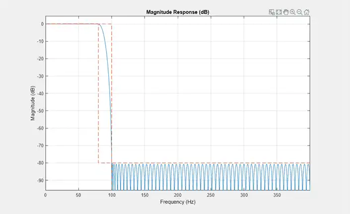
The specifications for the filter determine that a transition band of 20 Hz is acceptable between 80 and 100 Hz and that the minimum attenuation for out of band components is 80 dB. Also that the maximum distortion for the components of interest is 0.05 dB (half the peak-to-peak passband ripple). An equiripple filter that meets these specs can be easily obtained by the fdesign interface.

eqrDecim = design(fdDecim,'equiripple', 'SystemObject', true);
measure(eqrDecim)

ans = 

Sample Rate      : 800 Hz     
Passband Edge    : 80 Hz      
3-dB Point       : 85.621 Hz  
6-dB Point       : 87.8492 Hz 
Stopband Edge    : 100 Hz     
Passband Ripple  : 0.092414 dB
Stopband Atten.  : 80.3135 dB 
Transition Width : 20 Hz

Visualize the magnitude response confirms that the filter is an equiripple filter.

fvtool(eqrDecim)

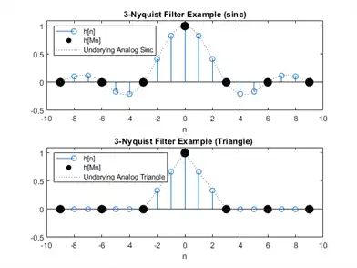
Nyquist Filters and Interpolation Consistency

A digital convolution filter $h$ is called an L-th Nyquist filter if it is vanishing periodically every $L$ samples, except the center index. In other words, the sampling $h$ by a factor of $L$ yields an impulse:

$h[kL] = \delta_k$

The $L$ -th band ideal lowpass, $h[m] = sinc(\frac{m}{L})$ , for example, is $L$ -th Nyquist filter. Another example is a triangular window.

L=3;
t = linspace(-3*L,3*L,1024);
n = (-3*L:3*L);
hLP = @(t) sinc(t/L);
hTri = @(t) (1-abs(t/L)).*(abs(t/L)<=1);

plot_nyquist_filter(t,n,hLP,hTri,L);

The function designMultirateFIR yields Nyquist filters, since it is based on weighted and truncated versions of ideal Nyquist filters.

Nyquist filters are efficient to implement since an L-th fraction of the coefficients in these filters are zero, which reduces the number of required multiplications. This feature makes these filters efficient for both decimation and interpolation.

Interpolation Consistency

Nyquist filters retain the sample values of the input even after filtering. This behavior, which is called interpolation consistency, is not true in general, as will be shown below.

Interpolation consistency holds in Nyquist filter, since the coefficients equal to zero every L samples (except for at the center). The proof is straightforward. Assume that $x_L$ is the upsampled version of $x$ (with zeros inserted between samples) so that $x_L[Ln]=x[n]$ , and that $y=h*x_L$ is the interpolated signal. Sample $y$ uniformly and get the following equation.

$y[nL] = (h*x_L)[Ln] = \sum_k h[Ln-k] x_L[k] = \sum_m \underbrace{h[Ln-Lm]}_{\delta[L(n-m)]} x_L[Lm] = x_L[Ln] = x[n]$

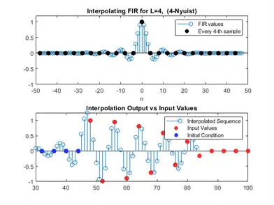
Let us examine the effect of using a Nyquist filter for interpolation. The designMultirateFIR function produces Nyquist filters. As you can see in the depiction below, the input values coincide with the interpolated values.

% Generate input
n = (0:20)';
xInput = (n<=10).*cos(pi*0.05*n).*(-1).^n;

L = 4;
hNyq = designMultirateFIR(L,1);
firNyq = dsp.FIRInterpolator(L,hNyq);
xIntrNyq = firNyq(xInput);
release(firNyq);
plot_shape_and_response(hNyq,xIntrNyq,xInput,L,num2str(L)+"-Nyuist");

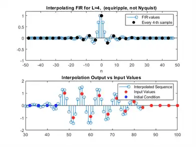
This is not the case for other lowpass filters such as equiripple designs, as seen in the figure below. Note that the interpolated sequence does not coincide with the low-rate input values. On the other hand, distortion may be lower in non-Nyquist filters, as a tradeoff for interpolation consistency.

hNotNyq = firpm(length(hNyq)-1,[0 1/L 1.5/L 1],[1 1 0 0]);
hNotNyq = hNotNyq/max(hNotNyq); % Adjust gain
firIntrNotNyq = dsp.FIRInterpolator(L,hNotNyq);
xIntrNotNyq= firIntrNotNyq(xInput);
release(firIntrNotNyq);

plot_shape_and_response(hNotNyq,xIntrNotNyq,xInput,L,"equiripple, not Nyquist");

Matlabsolutions.com provides guaranteed satisfaction with a commitment to complete the work within time. Combined with our meticulous work ethics and extensive domain experience, We are the ideal partner for all your homework/assignment needs. We pledge to provide 24*7 support to dissolve all your academic doubts. We are composed of 300+ esteemed Matlab and other experts who have been empanelled after extensive research and quality check.

Matlabsolutions.com provides undivided attention to each Matlab assignment order with a methodical approach to solution. Our network span is not restricted to US, UK and Australia rather extends to countries like Singapore, Canada and UAE. Our Matlab assignment help services include Image Processing Assignments, Electrical Engineering Assignments, Matlab homework help, Matlab Research Paper help, Matlab Simulink help. Get your work done at the best price in industry.