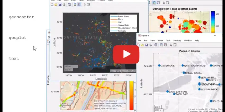
Plot Geographic Data on a Map using MATLAB

Introduction

MATLABSolutions demonstrate In this particular task, step-by-step guide to eographic displays offer valuable insights into data with latitude and longitude components. While you could plot this data in MATLAB using x and y coordinates, it would appear distorted and lack contextual information like political boundaries, roads, and other geographic features.

In MATLAB, geographic base maps provide this essential background context when plotting geographic data. These are tiled, multi-resolution web maps that enable you to pan and zoom across different regions of your plot, automatically loading new base map imagery as you navigate.

MATLAB simplifies the process of plotting data on a geographic base map within a MATLAB figure. There are two types of geographic maps you can create in a MATLAB figure:

• Geographic Axes Plot: This type behaves similarly to regular MATLAB axes. You can use plotting functions along with the hold on command to combine points, lines, text, and density plots in one geoaxes. For example, you can use geodensityplot, geoplot, and geoscatter to visualize density, line, and point data, respectively. You can then customize the view by changing the basemap and limits, and adding annotations like text, a legend, and a title.
• Geographic Bubble Chart: This specialized chart type can represent a continuous variable by bubble size and a categorical variable by bubble color. It provides both bubble and categorical legends.

MATLAB’s base maps for global and regional scales are loaded from the web by default, but you can also download the data from MATLAB Add-Ons for offline use. Additionally, web maps with street-level data, topography, or other specialized base layers can be loaded from third-party sources. You can easily add these web maps using the addCustomBasemap function available in the Mapping Toolbox.

These functions for overlaying latitude and longitude data on web map base layers are readily available in MATLAB. For more advanced needs, the Mapping Toolbox offers additional functions for visualizing data in other projected coordinate systems, converting between systems, and performing geodesy calculations such as calculating distances and areas. It also allows you to read and write data between various standard geographic file types like shapefiles, GPX files, and GeoTIFF files.

Matlabsolutions.com provides guaranteed satisfaction with a commitment to complete the work within time. Combined with our meticulous work ethics and extensive domain experience, We are the ideal partner for all your homework/assignment needs. We pledge to provide 24*7 support to dissolve all your academic doubts. We are composed of 300+ esteemed Matlab and other experts who have been empanelled after extensive research and quality check.

Matlabsolutions.com provides undivided attention to each Matlab assignment order with a methodical approach to solution. Our network span is not restricted to US, UK and Australia rather extends to countries like Singapore, Canada and UAE. Our Matlab assignment help services include Image Processing Assignments, Electrical Engineering Assignments, Matlab homework help, Matlab Research Paper help, Matlab Simulink help. Get your work done at the best price in industry.