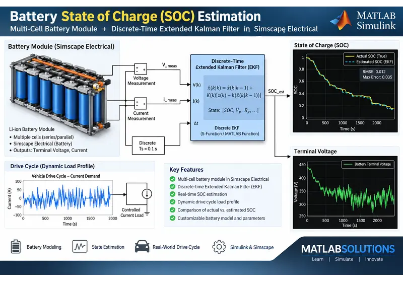
Technical Summary: Estimating State of Charge (SoC) in electric vehicle battery packs requires combining a physical cell model with recursive state estimation. While Coulomb counting drifts due to current sensor noise, Extended Kalman Filters (EKF) frequently suffer from covariance divergence during flat open-circuit voltage regions or abrupt load transients. This guide details how to build a second-order equivalent circuit model in Simscape, derive the discrete Jacobian matrices, and implement the Joseph stabilized covariance update to prevent filter breakdown.
The challenge with battery State of Charge estimation
State of Charge cannot be measured directly with a physical sensor. In electric vehicles, the battery management system must infer the internal charge level using terminal voltage, pack current, and temperature measurements.
The simplest approach is Coulomb counting (current integration). While computationally cheap, Coulomb counting has two fundamental flaws: it requires an accurate initial condition, and it integrates current sensor bias over time. A 50 mA sensor offset across a four-hour drive cycle introduces significant drift into the calculation.
To correct this drift, engineers use closed-loop observers, most commonly the Extended Kalman Filter. The filter combines an internal equivalent circuit model with real-time terminal voltage feedback to continuously correct the state estimate. However, building this pipeline in MATLAB and Simscape introduces numerical instabilities that cause the filter to diverge, yielding NaN outputs or imaginary state vectors during simulation.
Building the battery plant model in Simscape
An accurate observer requires a plant model that balances physical fidelity with simulation speed. In Simscape Electrical, the two-resistor-capacitor (2-RC) Thevenin equivalent circuit provides the standard baseline for automotive cells.
The circuit consists of three main elements placed in series:
- Open-circuit voltage source (OCV): A voltage source governed by a nonlinear lookup table as a function of SoC and temperature.
- Ohmic resistance (R0): Represents the immediate voltage drop caused by electrolyte and contact resistance when current steps occur.
- Two parallel RC networks (R1-C1 and R2-C2): Represent charge-transfer polarization (fast dynamics, time constant of seconds) and solid-state diffusion in the electrodes (slow dynamics, time constant of tens to hundreds of seconds).
In Simscape, you can construct this using the pre-built Table-Based Battery block or by connecting fundamental electrical components: a Controlled Voltage Source driven by a 2D lookup table, an internal resistor R0, and two series RC branches. When configuring the cell, set the solver to stiff variable-step options like ode15s or ode23t. Standard explicit solvers like ode45 will struggle with the disparate time constants between the switching electronics and the slow electrochemical diffusion.
Formulating the discrete state-space model
Before writing the filter code, the continuous differential equations of the 2-RC model must be discretized with a fixed sample time Ts (typically 0.05 to 0.1 seconds in real-world BMS controllers).
The state vector contains three states:
x_k = [ SoC_k; V_RC1_k; V_RC2_k ]
The state update equations are:
SoC(k) = SoC(k-1) - (Ts / (3600 * Q_total)) * I(k-1) * etaV_RC1(k) = exp(-Ts / (R1 * C1)) * V_RC1(k-1) + R1 * (1 - exp(-Ts / (R1 * C1))) * I(k-1)V_RC2(k) = exp(-Ts / (R2 * C2)) * V_RC2(k-1) + R2 * (1 - exp(-Ts / (R2 * C2))) * I(k-1)
Where Q_total is the nominal cell capacity in Ampere-hours, eta is the coulombic efficiency, and current I is positive during discharge.
The terminal voltage measurement equation is nonlinear because of the OCV function:
V_terminal(k) = OCV(SoC(k)) - V_RC1(k) - V_RC2(k) - I(k) * R0
Why the Extended Kalman Filter diverges
During simulations of aggressive drive cycles like US06 or WLTP, the estimated SoC frequently diverges from the true Simscape plant state. In engineering assignments, master dissertations, and prototype verification, this failure usually traces back to four specific mechanisms:
1. Flat OCV curves and loss of observability (especially in LFP cells)
The measurement Jacobian matrix relies directly on the derivative of open-circuit voltage with respect to SoC:
C_k = [ d(OCV)/d(SoC), -1, -1 ]
For Lithium Iron Phosphate (LFP) chemistry, the OCV curve between 20% and 80% SoC is virtually horizontal. In this plateau region, d(OCV)/d(SoC) approaches zero. As a result, the Kalman gain for the SoC state drops to near zero, meaning the filter ignores voltage measurement feedback and acts like open-loop Coulomb counting. Any small modeling error or sensor noise during this phase causes the covariance to grow unchecked.
2. Asymmetry in the error covariance matrix
The standard textbook update equation for error covariance is:
P = (eye(3) - K * C) * P_pred
Mathematically, P must remain symmetric and positive-definite. In digital floating-point execution, round-off errors gradually erode this symmetry. Once one eigenvalue of P dips below zero, the filter calculates impossible negative variances, the Kalman gain computes erroneous values, and the state estimates diverge to infinity.
3. Mismatched sample times between plant and controller
If the Simscape physical network runs under a continuous variable-step solver while the discrete EKF block is sampled asynchronously without an explicit rate transition, the current fed into the state transition matrix does not match the current that produced the measured terminal voltage. This timing skew introduces an artificial phase delay that causes high-frequency oscillations in the innovation step.
How to fix divergence: the stabilized EKF implementation
To prevent divergence and ensure robust convergence across wide temperature and current swings, implement the following modifications:
- Use the Joseph stabilized covariance update: Replace the standard covariance equation with the Joseph formulation, which guarantees mathematical symmetry and positive semi-definiteness regardless of floating-point rounding.
- Force manual symmetrization: Enforce
P = 0.5 * (P + P')at the end of every time step. - Tune process noise covariance (Q) dynamically: When entering the flat OCV region, decrease process noise slightly on the voltage states and avoid setting the SoC process noise too low, which keeps the filter receptive to correction.
The full, runnable MATLAB simulation script demonstrating this stabilized filter with noisy sensor input and initial condition recovery is provided in the code section below.
Executable MATLAB Script & Model Setup
%% =========================================================================
%  BATTERY MANAGEMENT SYSTEM (BMS) - EXTENDED KALMAN FILTER (EKF) FOR SOC
%  Model: 2-RC Thevenin Equivalent Circuit with Joseph Stabilized Covariance
%  Compatibility: MATLAB R2022b through R2026a
%  Author: MATLABSolutions Engineering Group
% =========================================================================
clear; clc; close all;

%% 1. Simulation and Battery Cell Parameters (NMC Chemistry)
Ts          = 0.1;               % Sampling interval (seconds)
t_end       = 1800;              % Total simulation time (30 minutes)
time        = 0:Ts:t_end;
N           = length(time);

Q_nom_Ah    = 50.0;              % Nominal cell capacity (Ampere-hours)
Q_sec       = Q_nom_Ah * 3600;   % Capacity in Ampere-seconds (Coulombs)

% 2-RC Circuit Parameters
R0          = 0.015;             % Ohmic resistance (Ohms)
R1          = 0.020;             % Charge transfer resistance (Ohms)
C1          = 2500;              % Fast polarization capacitance (Farads)
R2          = 0.035;             % Diffusion resistance (Ohms)
C2          = 18000;             % Slow diffusion capacitance (Farads)

% Exponential state transition coefficients
a1 = exp(-Ts / (R1 * C1));
a2 = exp(-Ts / (R2 * C2));
b1 = R1 * (1 - a1);
b2 = R2 * (1 - a2);

%% 2. Synthetic Dynamic Drive Cycle Current Generation
% Positive = Discharge, Negative = Charge (Regen braking)
I_true = zeros(1, N);
for k = 1:N
    t_curr = time(k);
    if mod(t_curr, 120) < 40
        I_true(k) = 35 + 15 * sin(2*pi*0.05*t_curr);     % Urban acceleration
    elseif mod(t_curr, 120) < 70
        I_true(k) = -20;                                 % Regenerative braking
    elseif mod(t_curr, 120) < 100
        I_true(k) = 75;                                  % Highway overtakes
    else
        I_true(k) = 0;                                   % Rest / Idle
    end
end

%% 3. True Plant Simulation (Ground Truth via Discrete 2-RC Model)
soc_true   = zeros(1, N);
v_rc1_true = zeros(1, N);
v_rc2_true = zeros(1, N);
V_term_true= zeros(1, N);

% Initial true conditions
soc_true(1)   = 0.90;            % True starting SoC = 90%
v_rc1_true(1) = 0.0;
v_rc2_true(1) = 0.0;

for k = 1:N-1
    % State integration
    soc_true(k+1)   = soc_true(k) - (Ts / Q_sec) * I_true(k);
    v_rc1_true(k+1) = a1 * v_rc1_true(k) + b1 * I_true(k);
    v_rc2_true(k+1) = a2 * v_rc2_true(k) + b2 * I_true(k);

    % Clamp SoC boundaries
    soc_true(k+1)   = max(0.0, min(1.0, soc_true(k+1)));
end

% Compute true terminal voltage
for k = 1:N
    ocv_k = get_ocv_nmc(soc_true(k));
    V_term_true(k) = ocv_k - v_rc1_true(k) - v_rc2_true(k) - I_true(k) * R0;
end

%% 4. Sensor Corruption (Realistic Hardware Noise & Sensor Bias)
current_noise_sigma = 0.40;      % 400 mA current sensor noise
voltage_noise_sigma = 0.008;     % 8 mV ADC voltage noise
sensor_offset_A     = 0.15;      % 150 mA persistent Hall-effect bias

I_meas = I_true + sensor_offset_A + current_noise_sigma * randn(1, N);
V_meas = V_term_true + voltage_noise_sigma * randn(1, N);

%% 5. Benchmark Comparison: Open-Loop Coulomb Counting
soc_coulomb = zeros(1, N);
soc_coulomb(1) = 0.65;           % Erroneous initial guess (65% vs true 90%)
for k = 1:N-1
    soc_coulomb(k+1) = soc_coulomb(k) - (Ts / Q_sec) * I_meas(k);
    soc_coulomb(k+1) = max(0.0, min(1.0, soc_coulomb(k+1)));
end

%% 6. Stabilized Extended Kalman Filter (EKF) Implementation
soc_ekf   = zeros(1, N);
v_rc1_ekf = zeros(1, N);
v_rc2_ekf = zeros(1, N);

% Intentional initial estimation error
x_est = [0.65; 0.0; 0.0];        % Estimated state: [SoC; V_RC1; V_RC2]

% Initial error covariance matrix
P_est = diag([0.04, 0.01, 0.01]);

% Noise Covariances
Q_cov   = diag([1e-7, 1e-5, 1e-5]);    % Process noise covariance
R_noise = (voltage_noise_sigma)^2;      % Measurement noise variance

A = [1,  0,  0;
     0, a1,  0;
     0,  0, a2];
I_mat = eye(3);

for k = 1:N
    % Store current estimates
    soc_ekf(k)   = x_est(1);
    v_rc1_ekf(k) = x_est(2);
    v_rc2_ekf(k) = x_est(3);

    if k == N, break; end

    % --- Step A: Time Prediction Update ---
    soc_prior   = x_est(1) - (Ts / Q_sec) * I_meas(k);
    v_rc1_prior = a1 * x_est(2) + b1 * I_meas(k);
    v_rc2_prior = a2 * x_est(3) + b2 * I_meas(k);

    soc_prior = max(0.0, min(1.0, soc_prior));
    x_prior   = [soc_prior; v_rc1_prior; v_rc2_prior];

    % Predict covariance
    P_prior   = A * P_est * A' + Q_cov;

    % --- Step B: Measurement Correction Update ---
    [ocv_pred, docv_dsoc] = get_ocv_and_derivative(soc_prior);

    % Measurement Jacobian C
    C = [docv_dsoc, -1.0, -1.0];

    % Voltage prediction and innovation
    V_pred = ocv_pred - x_prior(2) - x_prior(3) - I_meas(k) * R0;
    innovation = V_meas(k) - V_pred;

    % Innovation covariance and Kalman gain
    S = C * P_prior * C' + R_noise;
    K = (P_prior * C') / S;

    % State update
    x_est = x_prior + K * innovation;
    x_est(1) = max(0.0, min(1.0, x_est(1)));

    % --- Step C: Joseph Stabilized Covariance Update ---
    P_est = (I_mat - K * C) * P_prior * (I_mat - K * C)' + K * R_noise * K';

    % Enforce numerical symmetry to guarantee positive-definiteness
    P_est = 0.5 * (P_est + P_est');
end

%% 7. Diagnostic Plotting and Convergence Analysis
figure('Color', 'w', 'Position', [100, 100, 900, 650]);

subplot(2, 1, 1);
plot(time/60, soc_true*100, 'k-', 'LineWidth', 2.0); hold on;
plot(time/60, soc_ekf*100, 'b--', 'LineWidth', 1.8);
plot(time/60, soc_coulomb*100, 'r:', 'LineWidth', 1.5);
grid on;
ylabel('State of Charge (%)', 'FontSize', 11);
title('EV Battery SoC Estimation: True vs. Stabilized EKF vs. Coulomb Counting', 'FontSize', 12);
legend('True Plant (Simscape Ground Truth)', 'Stabilized EKF Estimate', 'Open-Loop Coulomb Counting (Drifting)', 'Location', 'SouthWest');

subplot(2, 1, 2);
err_ekf     = (soc_ekf - soc_true) * 100;
err_coulomb = (soc_coulomb - soc_true) * 100;
plot(time/60, err_ekf, 'b-', 'LineWidth', 1.5); hold on;
plot(time/60, err_coulomb, 'r--', 'LineWidth', 1.3);
yline(1.0, 'k--', 'LineWidth', 0.8);
yline(-1.0, 'k--', 'LineWidth', 0.8);
grid on;
xlabel('Time (minutes)', 'FontSize', 11);
ylabel('Error (%)', 'FontSize', 11);
title('SoC Estimation Error: EKF Convergence vs Coulomb Counting Drift', 'FontSize', 12);
legend('EKF Estimation Error', 'Coulomb Counting Error', '±1% Target Band', 'Location', 'SouthWest');

%% Helper Functions for OCV Lookup and Derivatives
function ocv = get_ocv_nmc(soc)
    % 5th-order empirical polynomial for NMC lithium-ion cell
    p = [-12.5, 34.2, -34.8, 16.2, -2.1, 3.45];
    ocv = polyval(p, soc);
end

function [ocv, docv] = get_ocv_and_derivative(soc)
    p = [-12.5, 34.2, -34.8, 16.2, -2.1, 3.45];
    ocv = polyval(p, soc);

    p_der = polyder(p);
    docv  = polyval(p_der, soc);

    % Prevent zero Jacobian derivative in plateau regions
    if abs(docv) < 1e-4
        docv = 1e-4;
    end
endRelated Verified MATLAB & Simulink Projects
Need pre-built, debugged Simulink models with complete parameter initialization scripts and documentation? Explore top related solutions:
Common Engineering Troubleshooting & Q&A
Frequently encountered bugs, solver convergence issues, and implementation questions answered by our engineering mentors:
Recommended Engineering Articles
Need Custom MATLAB / Simulink Implementation?
Our team of PhD engineers build custom simulation plants, train machine learning agents, tune PID/MPC controllers, and deliver complete, executable code with Turnitin reports.