1. Why Standard AI Fails on Real-World Physics Problems
If you've ever tried training a standard deep learning model to predict fluid dynamics, structural stress, or heat transfer, you've likely hit a wall. Standard neural networks excel at recognizing patterns in images or text, but when applied to physical systems, they fail in predictable ways:
- They demand unrealistic amounts of data: Gathering thousands of clean sensor readings across an entire physical component is rarely feasible or affordable.
- They break basic laws of physics: A standard network will happily predict negative energy, mass appearing out of nowhere, or fluid teleportation simply because the numbers fit the curve.
- They crumble outside the training range: The moment your machine operates slightly hotter or faster than the training set, predictions drift into nonsensical territory.
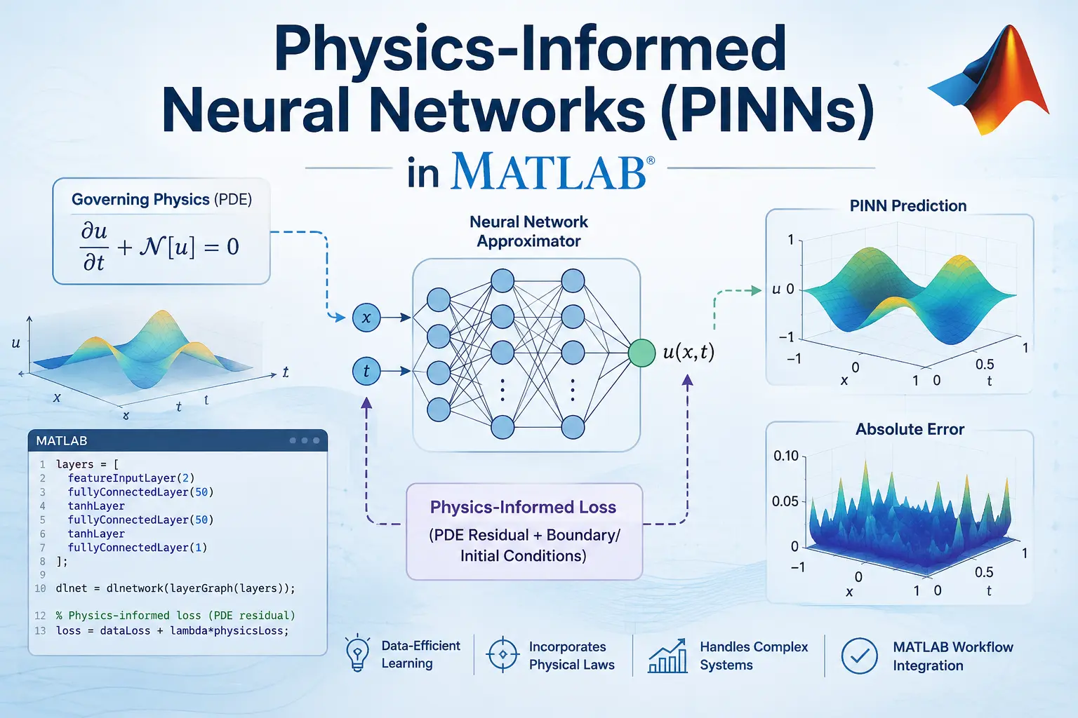
This is where Physics-Informed Neural Networks (PINNs) step in. Instead of forcing an AI to blindly guess physical behavior from raw data alone, a PINN bakes differential equations directly into the network's learning process. The model essentially acts as a mesh-free solver that respects physical conservation laws from day one.
2. How PINNs Work Under the Hood
Think of a PINN as a neural network operating under a strict supervisor. The supervisor doesn't just check if the model's guess matches known data points—it also tests whether the guess obeys the differential equations governing the physical system.
Mathematically, we set up our loss function as a balance between four distinct components:
Total Loss = (Data Loss) + (Initial Condition Loss) + (Boundary Loss) + (Physics Residual Loss)
- Data Loss: Penalizes discrepancies between network predictions and real-world sensor measurements.
- Initial & Boundary Losses: Ensure the solution honors starting conditions (like initial temperature) and physical borders (like insulated walls).
- Physics Residual Loss: Evaluates how closely the prediction satisfies the partial differential equation (PDE) using MATLAB's automatic differentiation.
3. Step-by-Step Implementation in MATLAB
Let's build a working PINN in MATLAB to solve a classic engineering problem: 1D Transient Heat Conduction governed by the equation:
∂u/∂t - α * ∂²u/∂x² = 0
Step 1: Setting Up Domain Points & Formatting for Automatic Differentiation
First, we generate collocation points across our domain where the network will evaluate the physical PDE residual, alongside boundary and initial condition points.
% Clear workspace and set physical parameters
clear; clc; close all;
alpha = 0.01; % Thermal diffusivity coefficient

% 1. Interior collocation points (where physics laws are enforced)
N_coll = 2500;
x_coll = rand(N_coll, 1);
t_coll = rand(N_coll, 1);

% 2. Initial state points (t = 0, u(x,0) = sin(pi*x))
N_ic = 250;
x_ic = linspace(0, 1, N_ic)';
t_ic = zeros(N_ic, 1);
u_ic = sin(pi * x_ic);

% 3. Boundary points (Fixed zero temperature at ends x=0 and x=1)
N_bc = 250;
t_bc = linspace(0, 1, N_bc)';
x_bc0 = zeros(N_bc, 1);
x_bc1 = ones(N_bc, 1);

% Format into dlarray for MATLAB automatic differentiation
X_coll = dlarray([x_coll, t_coll]', 'CB');
X_ic   = dlarray([x_ic, t_ic]', 'CB');
U_ic   = dlarray(u_ic', 'CB');

X_bc0  = dlarray([x_bc0, t_bc]', 'CB');
X_bc1  = dlarray([x_bc1, t_bc]', 'CB');
U_bc   = dlarray(zeros(N_bc, 1)', 'CB');
Step 2: Defining the Neural Network Architecture
We use a Multi-Layer Perceptron (MLP) with smooth tanh activation functions. Avoid ReLU here—its second derivative is zero, which kills the physics gradient computation!
% Define multi-layer perceptron
layers = [
    featureInputLayer(2, 'Name', 'input_space_time')
    fullyConnectedLayer(40, 'Name', 'hidden1')
    tanhLayer('Name', 'act1')
    fullyConnectedLayer(40, 'Name', 'hidden2')
    tanhLayer('Name', 'act2')
    fullyConnectedLayer(40, 'Name', 'hidden3')
    tanhLayer('Name', 'act3')
    fullyConnectedLayer(1, 'Name', 'predicted_temperature')
];

net = dlnetwork(layers);
Step 3: Building the Physics-Informed Custom Loss Function
Here is where the magic happens. We leverage dlgradient to calculate spatial and temporal partial derivatives automatically.
function [loss, gradients] = pinnLoss(net, X_coll, X_ic, U_ic, X_bc0, X_bc1, U_bc, alpha)
    % A. Initial Condition Loss
    U_ic_hat = forward(net, X_ic);
    loss_IC = mean((U_ic_hat - U_ic).^2, 'all');

    % B. Boundary Condition Loss
    U_bc0_hat = forward(net, X_bc0);
    U_bc1_hat = forward(net, X_bc1);
    loss_BC = mean((U_bc0_hat - U_bc).^2, 'all') + mean((U_bc1_hat - U_bc).^2, 'all');

    % C. Physics PDE Residual Loss via Automatic Differentiation
    x_nodes = X_coll(1, :);
    t_nodes = X_coll(2, :);

    u_hat = forward(net, X_coll);

    % Compute first-order partial derivatives
    u_t = dlgradient(sum(u_hat, 'all'), t_nodes, 'EnableSearch', true);
    u_x = dlgradient(sum(u_hat, 'all'), x_nodes, 'EnableSearch', true);

    % Compute second-order spatial derivative
    u_xx = dlgradient(sum(u_x, 'all'), x_nodes, 'EnableSearch', true);

    % Heat equation residual: u_t - alpha * u_xx = 0
    pde_residual = u_t - alpha * u_xx;
    loss_physics = mean(pde_residual.^2, 'all');

    % Total weighted loss
    loss = 2.0 * loss_IC + 2.0 * loss_BC + 1.0 * loss_physics;

    % Compute backpropagation gradients wrt weights
    gradients = dlgradient(loss, net.Learnables);
end
Step 4: Training Optimization Loop
% Optimization parameters
maxEpochs = 4000;
lr = 1e-3;
avgG = []; avgSQG = [];

fprintf('Starting PINN training loop...\n');
for epoch = 1:maxEpochs
    % Evaluate loss and parameter gradients
    [loss, grads] = dlfeval(@pinnLoss, net, X_coll, X_ic, U_ic, X_bc0, X_bc1, U_bc, alpha);

    % Update network weights using ADAM algorithm
    [net, avgG, avgSQG] = adamupdate(net, grads, avgG, avgSQG, epoch, lr);

    % Print progress every 500 epochs
    if mod(epoch, 500) == 0 || epoch == 1
        fprintf('Epoch %4d | Total PINN Loss: %.6e\n', epoch, extractdata(loss));
    end
end
fprintf('Training complete!\n');
4. Troubleshooting Common PINN Pitfalls in MATLAB
| Issue | Why It Happens | How to Fix in MATLAB |
|---|---|---|
| Zero Physics Gradient | Using ReLU or non-differentiable activations | Switch all activation layers to smooth functions like tanh or swish. |
| Imbalanced Learning | Boundary loss dwarfed by physics loss | Multiply initial/boundary terms by higher weight factors in pinnLoss. |
| Slow Convergence | ADAM gets stuck near local minima | Pass trained network parameters into an L-BFGS optimizer via fmincon for final polishing. |
Related Verified MATLAB & Simulink Projects
Need pre-built, debugged Simulink models with complete parameter initialization scripts and documentation? Explore top related solutions:
Common Engineering Troubleshooting & Q&A
Frequently encountered bugs, solver convergence issues, and implementation questions answered by our engineering mentors:
Recommended Engineering Articles
Need Custom MATLAB / Simulink Implementation?
Our team of PhD engineers build custom simulation plants, train machine learning agents, tune PID/MPC controllers, and deliver complete, executable code with Turnitin reports.