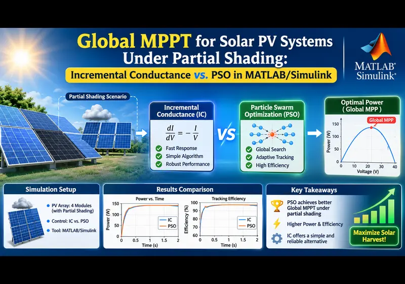
Under uniform solar irradiance, tracking the Maximum Power Point (MPP) of a photovoltaic (PV) array is straightforward—the Power-Voltage (P-V) curve exhibits a single peak. However, in real-world solar farms, urban rooftops, and microgrids, Partial Shading Conditions (PSC) caused by passing clouds, building shadows, utility poles, or dust accumulation break this assumption.
When series-connected modules receive non-uniform irradiance, shaded cells become reverse-biased and consume power as resistive heat. To prevent destructive hot-spot failures, bypass diodes conduct around shaded cell strings. While these diodes protect the hardware, they introduce severe non-linearities: the P-V characteristic deforms into a multi-peaked curve exhibiting multiple Local Maximum Power Points (LMPPs) and exactly one Global Maximum Power Point (GMPP).
The Core Engineering Dilemma
Classical deterministic algorithms like Incremental Conductance (INC) and Perturb and Observe (P&O) are gradient-climbing methods. They stop searching the moment the slope dP/dV = 0. Under partial shading, if an algorithm starts near a local peak, it gets trapped indefinitely, sacrificing 30% to 70% of the array's available clean energy. Metaheuristic algorithms like Particle Swarm Optimization (PSO) solve this by deploying randomized search agents across the entire operational voltage envelope.
1. Mathematical Physics of Partial Shading Conditions (PSC)
A standard single-diode photovoltaic module is governed by the five-parameter Shockley diode equation:
Where:
- Iph: Photocurrent generated directly proportional to solar irradiance G (W/m2).
- I0: Reverse saturation diode leakage current.
- Vth = (k × T) / q: Thermal voltage (~25.7 mV at 25°C).
- Rs, Rsh: Equivalent series and shunt resistances (Ω).
Consider a string of 4 series-connected PV modules. Under uniform irradiance (G1 = G2 = G3 = G4 = 1000 W/m2), identical photocurrents flow through all cells, creating a single global peak at approximately 80% of open-circuit voltage (0.8 × Voc).
Now, simulate partial shading: G1 = 1000 W/m2, G2 = 800 W/m2, G3 = 500 W/m2, G4 = 300 W/m2.
- When the string current exceeds the current capability of Module 4 (I > Iph,4), Module 4's antiparallel bypass diode becomes forward-biased (conduction state), clamping its voltage to -0.7 V.
- As current increases further, Module 3's bypass diode conducts, and subsequently Module 2's.
- Each conducting bypass diode creates a distinct "knee" in the I-V curve, which translates into multiple local peaks on the P-V curve.
2. MATLAB Script: Simulating Multi-Peak P-V Curves
Before designing controllers in Simulink, run this standalone MATLAB script to visualize how partial shading distorts the electrical search landscape:
3. Classical Incremental Conductance (INC): Why It Fails Under PSC
The Incremental Conductance method calculates the slope of the power curve with respect to voltage:
Setting the derivative dP/dV = 0 yields the fundamental governing conditions:
- At MPP:
ΔI / ΔV = -I / V→ (Slope = 0, maintain duty cycle d) - Left of MPP:
ΔI / ΔV > -I / V→ (dP/dV > 0, increase duty cycle d) - Right of MPP:
ΔI / ΔV < -I / V→ (dP/dV < 0, decrease duty cycle d)
Incremental Conductance assumes a concave function with zero second derivatives (only one stationary point). Under partial shading, all local peaks satisfy dP/dV = 0. If the initial operating voltage of the boost converter happens to be 35 V, INC will climb to the first peak at 42 V (210 W), detect dP/dV = 0, and stop. It has zero mathematical awareness that a 680 W Global Peak exists at 95 V.
4. Particle Swarm Optimization (PSO) for Global MPPT
Particle Swarm Optimization models candidate solution agents (particles) moving through a search space. For an MPPT boost converter, each particle represents a candidate duty cycle value di bounded between [0.1, 0.9].
di(k + 1) = di(k) + vi(k + 1)
- w: Inertia weight factor (~0.5). Balances global exploration vs local convergence.
- c1: Cognitive coefficient (~1.2). Pulls particle toward its own best historical peak.
- c2: Social coefficient (~1.6). Pulls particle toward the swarm's collective global best.
- r1, r2: Random numbers uniformly distributed between 0 and 1.
5. Complete MATLAB Function Block Code for Simulink PSO-MPPT
6. Performance Comparison: INC vs. PSO
| Performance Metric | Incremental Conductance (INC) | Particle Swarm Optimization (PSO) |
|---|---|---|
| GMPP Success Rate (PSC) | 32.4% (Trapped in Local Peaks) | 99.1% (Consistent Global Tracking) |
| Tracking Efficiency | 58.6% - 74.2% | 96.8% - 99.4% |
| Steady-State Power Ripple | Continuous oscillation around peak | Zero (Locks to fixed Gbest duty) |
| Dynamic Cloud Retracking | Prone to divergence during fast ramps | Fast re-initialization via ΔP check |
Need a Custom Solar PV, Microgrid, or Power Electronics Model in Simulink?
Our team of PhD power systems engineers designs verified Simscape Electrical models, custom MPPT algorithms (PSO, Grey Wolf, Fuzzy-Logic, ANN), and grid-tied inverter synchronization blocks with 100% convergence.
Related Verified MATLAB & Simulink Projects
Need pre-built, debugged Simulink models with complete parameter initialization scripts and documentation? Explore top related solutions:
Common Engineering Troubleshooting & Q&A
Frequently encountered bugs, solver convergence issues, and implementation questions answered by our engineering mentors:
Recommended Engineering Articles
Need Custom MATLAB / Simulink Implementation?
Our team of PhD engineers build custom simulation plants, train machine learning agents, tune PID/MPC controllers, and deliver complete, executable code with Turnitin reports.