Introduction: PID Controller Design

Contents

PID Overview

In this tutorial, we will consider the following unity-feedback system:

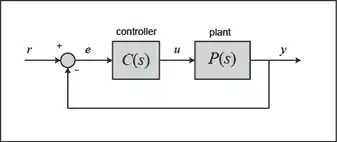
The output of a PID controller, which is equal to the control input to the plant, is calculated in the time domain from the feedback error as follows:

(1)

First, let's take a look at how the PID controller works in a closed-loop system using the schematic shown above. The variable () represents the tracking error, the difference between the desired output () and the actual output (). This error signal () is fed to the PID controller, and the controller computes both the derivative and the integral of this error signal with respect to time. The control signal () to the plant is equal to the proportional gain () times the magnitude of the error plus the integral gain () times the integral of the error plus the derivative gain () times the derivative of the error.

This control signal () is fed to the plant and the new output () is obtained. The new output () is then fed back and compared to the reference to find the new error signal (). The controller takes this new error signal and computes an update of the control input. This process continues while the controller is in effect.

The transfer function of a PID controller is found by taking the Laplace transform of Equation (1).

(2)

where  = proportional gain,  = integral gain, and  = derivative gain.

We can define a PID controller in MATLAB using a transfer function model directly, for example:

Kp = 1;
Ki = 1;
Kd = 1;

s = tf('s');
C = Kp + Ki/s + Kd*s

C =
 
  s^2 + s + 1
  -----------
       s
 
Continuous-time transfer function.

Alternatively, we may use MATLAB's pid object to generate an equivalent continuous-time controller as follows:

C = pid(Kp,Ki,Kd)

C =
 
             1          
  Kp + Ki * --- + Kd * s
             s          

  with Kp = 1, Ki = 1, Kd = 1
 
Continuous-time PID controller in parallel form.

Let's convert the pid object to a transfer function to verify that it yields the same result as above:

tf(C)

years =
 
  s^2 + s + 1
  -----------
       s
 
Continuous-time transfer function.

The Characteristics of the P, I, and D Terms

Increasing the proportional gain () has the effect of proportionally increasing the control signal for the same level of error. The fact that the controller will "push" harder for a given level of error tends to cause the closed-loop system to react more quickly, but also to overshoot more. Another effect of increasing  is that it tends to reduce, but not eliminate, the steady-state error.

The addition of a derivative term to the controller () adds the ability of the controller to "anticipate" error. With simple proportional control, if  is fixed, the only way that the control will increase is if the error increases. With derivative control, the control signal can become large if the error begins sloping upward, even while the magnitude of the error is still relatively small. This anticipation tends to add damping to the system, thereby decreasing overshoot. The addition of a derivative term, however, has no effect on the steady-state error.

The addition of an integral term to the controller () tends to help reduce steady-state error. If there is a persistent, steady error, the integrator builds and builds, thereby increasing the control signal and driving the error down. A drawback of the integral term, however, is that it can make the system more sluggish (and oscillatory) since when the error signal changes sign, it may take a while for the integrator to "unwind."

The general effects of each controller parameter (, , ) on a closed-loop system are summarized in the table below. Note, these guidelines hold in many cases, but not all. If you truly want to know the effect of tuning the individual gains, you will have to do more analysis, or will have to perform testing on the actual system.

Example Problem

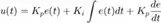
Suppose we have a simple mass-spring-damper system.

The governing equation of this system is

(3)

Taking the Laplace transform of the governing equation, we get

(4)

The transfer function between the input force  and the output displacement  then becomes

(5)

Let

    m = 1 kg
    b = 10 N s/m
    k = 20 N/m
    F = 1 N

Substituting these values into the above transfer function

(6)

The goal of this problem is to show how each of the terms, , , and , contributes to obtaining the common goals of:

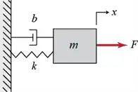
Open-Loop Step Response

Let's first view the open-loop step response. Create a new m-file and run the following code:

s = tf('s');
P = 1/(s^2 + 10*s + 20);
step(P)

The DC gain of the plant transfer function is 1/20, so 0.05 is the final value of the output to a unit step input. This corresponds to a steady-state error of 0.95, which is quite large. Furthermore, the rise time is about one second, and the settling time is about 1.5 seconds. Let's design a controller that will reduce the rise time, reduce the settling time, and eliminate the steady-state error.

Proportional Control

From the table shown above, we see that the proportional controller () reduces the rise time, increases the overshoot, and reduces the steady-state error.

The closed-loop transfer function of our unity-feedback system with a proportional controller is the following, where  is our output (equals ) and our reference  is the input:

(7)

Let the proportional gain () equal 300 and change the m-file to the following:

Kp = 300;
C = pid(Kp)
T = feedback(C*P,1)

t = 0:0.01:2;
step(T,t)

C =
 
  Kp = 300
 
P-only controller.


T =
 
        300
  ----------------
  s^2 + 10 s + 320
 
Continuous-time transfer function.

<img " src="../images/introduction-controlpid-02.png" alt="" width="90%" height="80%" />

The above plot shows that the proportional controller reduced both the rise time and the steady-state error, increased the overshoot, and decreased the settling time by a small amount.

Proportional-Derivative Control

Now, let's take a look at PD control. From the table shown above, we see that the addition of derivative control () tends to reduce both the overshoot and the settling time. The closed-loop transfer function of the given system with a PD controller is:

(8)

Let  equal 300 as before and let  equal 10. Enter the following commands into an m-file and run it in the MATLAB command window.

Kp = 300;
Kd = 10;
C = pid(Kp,0,Kd)
T = feedback(C*P,1)

t = 0:0.01:2;
step(T,t)

C =
 
             
  Kp + Kd * s
             

  with Kp = 300, Kd = 10
 
Continuous-time PD controller in parallel form.


T =
 
     10 s + 300
  ----------------
  s^2 + 20 s + 320
 
Continuous-time transfer function.

This plot shows that the addition of the derivative term reduced both the overshoot and the settling time, and had a negligible effect on the rise time and the steady-state error.

Proportional-Integral Control

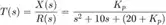
Before proceeding to PID control, let's investigate PI control. From the table, we see that the addition of integral control () tends to decrease the rise time, increase both the overshoot and the settling time, and reduces the steady-state error. For the given system, the closed-loop transfer function with a PI controller is:

(9)

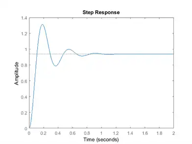
Let's reduce  to 30, and let  equal 70. Create a new m-file and enter the following commands.

Kp = 30;
Ki = 70;
C = pid (Kp, Ki)
T = feedback(C*P,1)

t = 0:0.01:2;
step(T,t)

C =
 
             1 
  Kp + Ki * ---
             s 

  with Kp = 30, Ki = 70
 
Continuous-time PI controller in parallel form.


T =
 
         30 s + 70
  ------------------------
  s^3 + 10 s^2 + 50 s + 70
 
Continuous-time transfer function.

Run this m-file in the MATLAB command window and you should generate the above plot. We have reduced the proportional gain () because the integral controller also reduces the rise time and increases the overshoot as the proportional controller does (double effect). The above response shows that the integral controller eliminated the steady-state error in this case.

Proportional-Integral-Derivative Control

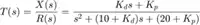
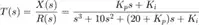
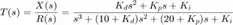
Now, let's examine PID control. The closed-loop transfer function of the given system with a PID controller is:

(10)

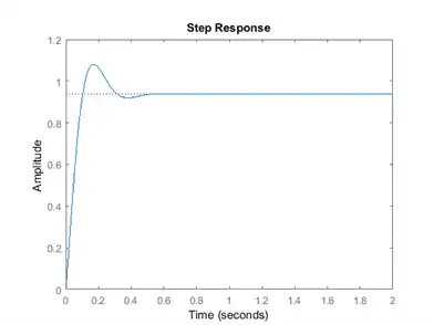
After several iterations of tuning, the gains  = 350,  = 300, and  = 50 provided the desired response. To confirm, enter the following commands to an m-file and run it in the command window. You should obtain the following step response.

Kp = 350;
Ki = 300;
Kd = 50;
C = pid(Kp,Ki,Kd)
T = feedback(C*P,1);

t = 0:0.01:2;
step(T,t)

C =
 
             1          
  Kp + Ki * --- + Kd * s
             s          

  with Kp = 350, Ki = 300, Kd = 50
 
Continuous-time PID controller in parallel form.

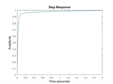
Now, we have designed a closed-loop system with no overshoot, fast rise time, and no steady-state error.

General Tips for Designing a PID Controller

When you are designing a PID controller for a given system, follow the steps shown below to obtain a desired response.

Lastly, please keep in mind that you do not need to implement all three controllers (proportional, derivative, and integral) into a single system, if not necessary. For example, if a PI controller meets the given requirements (like the above example), then you don't need to implement a derivative controller on the system. Keep the controller as simple as possible.

An example of tuning a PI controller on an actual physical system can be found at the following link. This example also begins to illustrate some challenges of implementing control, including: control saturation, integrator wind-up, and noise amplification.

Automatic PID Tuning

MATLAB provides tools for automatically choosing optimal PID gains which makes the trial and error process described above unnecessary. You can access the tuning algorithm directly using pidtune or through a nice graphical user interface (GUI) using pidTuner.

The MATLAB automated tuning algorithm chooses PID gains to balance performance (response time, bandwidth) and robustness (stability margins). By default, the algorithm designs for a 60-degree phase margin.

Let's explore these automated tools by first generating a proportional controller for the mass-spring-damper system by entering the command shown below. In the shown syntax, P is the previously generated plant model, and 'p' specifies that the tuner employ a proportional controller.

         pidTuner(P,'p')
         

The pidTuner GUI window, like that shown below, should appear.

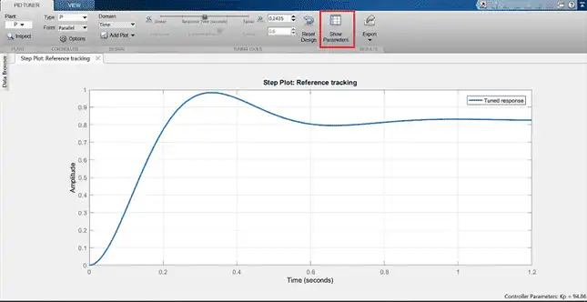
Notice that the step response shown is slower than the proportional controller we designed by hand. Now click on the Show Parameters button on the top right. As expected, the proportional gain, , is smaller than the one we employed,  = 94.86 < 300.

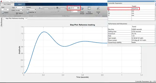
We can now interactively tune the controller parameters and immediately see the resulting response in the GUI window. Try dragging the Response Time slider to the right to 0.14 s, as shown in the figure below. This causes the response to indeed speed up, and we can see  is now closer to the manually chosen value. We can also see other performance and robustness parameters for the system. Note that before we adjusted the slider, the target phase margin was 60 degrees. This is the default for the pidTuner and generally provides a good balance between robustness and performance.

Now let's try designing a PID controller for our system. By specifying the previously designed or (baseline) controller, C, as the second parameter, pidTuner will design another PID controller (instead of P or PI) and will compare the response of the system with the automated controller with that of the baseline.

         pidTuner (P, C)
         

We see in the output window that the automated controller responds slower and exhibits more overshoot than the baseline. Now choose the Domain: Frequency option from the toolstrip, which reveals frequency domain tuning parameters.

Now type in 32 rad/s for Bandwidth and 90 deg for Phase Margin, to generate a controller similar in performance to the baseline. Keep in mind that a higher closed-loop bandwidth results in a faster rise time, and a larger phase margin reduces the overshoot and improves the system stability.

Finally, we note that we can generate the same controller using the command line tool pidtune instead of the pidTuner GUI employing the following syntax.

opts = pidtuneOptions('CrossoverFrequency',32,'PhaseMargin',90);
[C, info] = pidtune(P, 'pid', opts)

C =
 
             1          
  Kp + Ki * --- + Kd * s
             s          

  with Kp = 320, Ki = 796, Kd = 32.2
 
Continuous-time PID controller in parallel form.

info = 
  struct with fields:

                Stable: 1
    CrossoverFrequency: 32
           PhaseMargin: 90