Assess Neural Network Classifier Performance

Name: MATLABSOLUTIONS
Brand: MATLABSOLUTIONS
Rating: 4.9 (16783 reviews)

Create a feedforward neural network classifier with fully connected layers using fitcnet. Use validation data for early stopping of the training process to prevent overfitting the model. Then, use the object functions of the classifier to assess the performance of the model on test data.

Load and Preprocess Sample Data

This example uses the 1994 census data stored in census1994.mat. The data set consists of demographic information from the US Census Bureau that you can use to predict whether an individual makes over $50,000 per year.

Load the sample data census1994, which contains the training data adultdata and the test data adulttest. Preview the first few rows of the training data set.

load census1994
head(adultdata)

ans=8×15 table
    age       workClass          fnlwgt      education    education_num       marital_status           occupation        relationship     race      sex      capital_gain    capital_loss    hours_per_week    native_country    salary
    ___    ________________    __________    _________    _____________    _____________________    _________________    _____________    _____    ______    ____________    ____________    ______________    ______________    ______

    39     State-gov                77516    Bachelors         13          Never-married            Adm-clerical         Not-in-family    White    Male          2174             0                40          United-States     <=50K 
    50     Self-emp-not-inc         83311    Bachelors         13          Married-civ-spouse       Exec-managerial      Husband          White    Male             0             0                13          United-States     <=50K 
    38     Private             2.1565e+05    HS-grad            9          Divorced                 Handlers-cleaners    Not-in-family    White    Male             0             0                40          United-States     <=50K 
    53     Private             2.3472e+05    11th               7          Married-civ-spouse       Handlers-cleaners    Husband          Black    Male             0             0                40          United-States     <=50K 
    28     Private             3.3841e+05    Bachelors         13          Married-civ-spouse       Prof-specialty       Wife             Black    Female           0             0                40          Cuba              <=50K 
    37     Private             2.8458e+05    Masters           14          Married-civ-spouse       Exec-managerial      Wife             White    Female           0             0                40          United-States     <=50K 
    49     Private             1.6019e+05    9th                5          Married-spouse-absent    Other-service        Not-in-family    Black    Female           0             0                16          Jamaica           <=50K 
    52     Self-emp-not-inc    2.0964e+05    HS-grad            9          Married-civ-spouse       Exec-managerial      Husband          White    Male             0             0                45          United-States     >50K

Each row contains the demographic information for one adult. The last column, salary, shows whether a person has a salary less than or equal to $50,000 per year or greater than $50,000 per year.

Combine the education_num and education variables in both the training and test data to create a single ordered categorical variable that shows the highest level of education a person has achieved.

edOrder = unique(adultdata.education_num,"stable");
edCats = unique(adultdata.education,"stable");
[~,edIdx] = sort(edOrder);

adultdata.education = categorical(adultdata.education, ...
    edCats(edIdx),"Ordinal",true);
adultdata.education_num = [];

adulttest.education = categorical(adulttest.education, ...
    edCats(edIdx),"Ordinal",true);
adulttest.education_num = [];

Partition Training Data

Split the training data further using a stratified holdout partition. Create a separate validation data set to stop the model training process early. Reserve approximately 30% of the observations for the validation data set and use the rest of the observations to train the neural network classifier.

rng("default") % For reproducibility of the partition
c = cvpartition(adultdata.salary,"Holdout",0.30);
trainingIndices = training(c);
validationIndices = test(c);
tblTrain = adultdata(trainingIndices,:);
tblValidation = adultdata(validationIndices,:);

Train Neural Network

Train a neural network classifier by using the training set. Specify the salary column of tblTrain as the response and the fnlwgt column as the observation weights, and standardize the numeric predictors. Evaluate the model at each iteration by using the validation set. Specify to display the training information at each iteration by using the Verbose name-value argument. By default, the training process ends early if the validation cross-entropy loss is greater than or equal to the minimum validation cross-entropy loss computed so far, six times in a row. To change the number of times the validation loss is allowed to be greater than or equal to the minimum, specify the ValidationPatience name-value argument.

Mdl = fitcnet(tblTrain,"salary","Weights","fnlwgt", ...
    "Standardize",true,"ValidationData",tblValidation, ...
    "Verbose",1);

|==========================================================================================|
| Iteration  | Train Loss | Gradient   | Step       | Iteration  | Validation | Validation |
|            |            |            |            | Time (sec) | Loss       | Checks     |
|==========================================================================================|
|           1|    0.297812|    0.078920|    0.703981|    0.012127|    0.296816|           0|
|           2|    0.281110|    0.054594|    0.149850|    0.012486|    0.280132|           0|
|           3|    0.252648|    0.062041|    1.004181|    0.011339|    0.247863|           0|
|           4|    0.211868|    0.023567|    0.267214|    0.011319|    0.208988|           0|
|           5|    0.207039|    0.057528|    0.320942|    0.010288|    0.206781|           0|
|           6|    0.196838|    0.022492|    0.089842|    0.011197|    0.195583|           0|
|           7|    0.186133|    0.025551|    0.295975|    0.010426|    0.184900|           0|
|           8|    0.178779|    0.023714|    0.244525|    0.010237|    0.179370|           0|
|           9|    0.174531|    0.027149|    0.306182|    0.012911|    0.178175|           0|
|          10|    0.173217|    0.013365|    0.037475|    0.011084|    0.176371|           0|
|==========================================================================================|
| Iteration  | Train Loss | Gradient   | Step       | Iteration  | Validation | Validation |
|            |            |            |            | Time (sec) | Loss       | Checks     |
|==========================================================================================|
|          11|    0.168160|    0.016506|    0.307350|    0.010016|    0.170415|           0|
|          12|    0.164460|    0.025136|    0.473227|    0.011512|    0.165902|           0|
|          13|    0.162895|    0.014983|    0.473367|    0.010969|    0.164582|           0|
|          14|    0.160791|    0.005187|    0.113760|    0.011720|    0.162947|           0|
|          15|    0.159742|    0.004035|    0.138748|    0.010260|    0.162074|           0|
|          16|    0.159290|    0.005774|    0.108266|    0.010400|    0.161728|           0|
|          17|    0.158593|    0.004977|    0.152142|    0.010603|    0.161272|           0|
|          18|    0.157437|    0.003660|    0.193303|    0.010510|    0.160299|           0|
|          19|    0.156642|    0.007722|    0.430859|    0.010069|    0.160145|           0|
|          20|    0.155954|    0.001908|    0.121039|    0.010041|    0.159066|           0|
|==========================================================================================|
| Iteration  | Train Loss | Gradient   | Step       | Iteration  | Validation | Validation |
|            |            |            |            | Time (sec) | Loss       | Checks     |
|==========================================================================================|
|          21|    0.155824|    0.001645|    0.025159|    0.010557|    0.158992|           0|
|          22|    0.155486|    0.003232|    0.119915|    0.010829|    0.158731|           0|
|          23|    0.155398|    0.006845|    0.083105|    0.031846|    0.158963|           1|
|          24|    0.155261|    0.004374|    0.065660|    0.010762|    0.158816|           2|
|          25|    0.154955|    0.002505|    0.264106|    0.011437|    0.158687|           0|
|          26|    0.154799|    0.002183|    0.040876|    0.010903|    0.158538|           0|
|          27|    0.154466|    0.002881|    0.219478|    0.012409|    0.158033|           0|
|          28|    0.154250|    0.002724|    0.196190|    0.012062|    0.157980|           0|
|          29|    0.153918|    0.002189|    0.135392|    0.009862|    0.157605|           0|
|          30|    0.153707|    0.001449|    0.111574|    0.010851|    0.157456|           0|
|==========================================================================================|
| Iteration  | Train Loss | Gradient   | Step       | Iteration  | Validation | Validation |
|            |            |            |            | Time (sec) | Loss       | Checks     |
|==========================================================================================|
|          31|    0.153214|    0.002050|    0.528628|    0.010212|    0.157379|           0|
|          32|    0.152671|    0.002542|    0.488640|    0.010013|    0.156687|           0|
|          33|    0.152303|    0.004554|    0.223206|    0.010334|    0.156778|           1|
|          34|    0.152093|    0.002856|    0.121284|    0.010188|    0.156639|           0|
|          35|    0.151871|    0.003145|    0.135909|    0.010108|    0.156446|           0|
|          36|    0.151741|    0.001441|    0.225342|    0.010452|    0.156517|           1|
|          37|    0.151626|    0.002500|    0.396782|    0.010487|    0.156429|           0|
|          38|    0.151488|    0.005053|    0.148248|    0.010312|    0.156201|           0|
|          39|    0.151250|    0.002552|    0.110278|    0.009895|    0.155968|           0|
|          40|    0.151013|    0.002506|    0.123906|    0.010837|    0.155812|           0|
|==========================================================================================|
| Iteration  | Train Loss | Gradient   | Step       | Iteration  | Validation | Validation |
|            |            |            |            | Time (sec) | Loss       | Checks     |
|==========================================================================================|
|          41|    0.150821|    0.002536|    0.109515|    0.010627|    0.155742|           0|
|          42|    0.150509|    0.001418|    0.223296|    0.010561|    0.155648|           0|
|          43|    0.150340|    0.003437|    0.185351|    0.010131|    0.155435|           0|
|          44|    0.150280|    0.004746|    0.115075|    0.010432|    0.155797|           1|
|          45|    0.150194|    0.002758|    0.082143|    0.010068|    0.155575|           2|
|          46|    0.150061|    0.001122|    0.094288|    0.011405|    0.155334|           0|
|          47|    0.149978|    0.001259|    0.127677|    0.010628|    0.155305|           0|
|          48|    0.149879|    0.001523|    0.107816|    0.011331|    0.155044|           0|
|          49|    0.149749|    0.004572|    0.156869|    0.009953|    0.155043|           0|
|          50|    0.149617|    0.000965|    0.186502|    0.009702|    0.155106|           1|
|==========================================================================================|
| Iteration  | Train Loss | Gradient   | Step       | Iteration  | Validation | Validation |
|            |            |            |            | Time (sec) | Loss       | Checks     |
|==========================================================================================|
|          51|    0.149579|    0.001302|    0.062687|    0.010743|    0.155160|           2|
|          52|    0.149519|    0.001407|    0.086000|    0.010335|    0.155216|           3|
|          53|    0.149405|    0.001243|    0.147530|    0.009753|    0.155309|           4|
|          54|    0.149203|    0.002749|    0.186920|    0.010267|    0.155337|           5|
|          55|    0.149040|    0.001217|    0.310011|    0.012444|    0.155460|           6|
|==========================================================================================|

Use the information inside the TrainingHistory property of the object Mdl to check the iteration that corresponds to the minimum validation cross-entropy loss. The final returned model Mdl is the model trained at this iteration.

iteration = Mdl.TrainingHistory.Iteration;
valLosses = Mdl.TrainingHistory.ValidationLoss;
[~,minIdx] = min(valLosses);
iteration(minIdx)

ans = 49

Evaluate Test Set Performance

Evaluate the performance of the trained classifier Mdl on the test set adulttest by using the predict, loss, margin, and edge object functions.

Find the predicted labels and classification scores for the observations in the test set.

[labels,Scores] = predict(Mdl,adulttest);

Create a confusion matrix from the test set results. The diagonal elements indicate the number of correctly classified instances of a given class. The off-diagonal elements are instances of misclassified observations.

confusionchart(adulttest.salary,labels)

Compute the test set classification accuracy.

error = loss(Mdl,adulttest,"salary");
accuracy = (1-error)*100

accuracy = 85.1306

The neural network classifier correctly classifies approximately 85% of the test set observations.

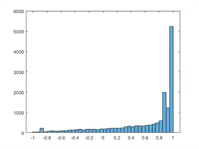
Compute the test set classification margins for the trained neural network. Display a histogram of the margins.

The classification margins are the difference between the classification score for the true class and the classification score for the false class. Because neural network classifiers return scores that are posterior probabilities, classification margins close to 1 indicate confident classifications and negative margin values indicate misclassifications.

m = margin(Mdl,adulttest,"salary");
histogram(m)

Use the classification edge, or mean of the classification margins, to assess the overall performance of the classifier.

meanMargin = edge(Mdl,adulttest,"salary")

meanMargin = 0.5983

Alternatively, compute the weighted classification edge by using observation weights.

weightedMeanMargin = edge(Mdl,adulttest,"salary", ...
    "Weight","fnlwgt")

weightedMeanMargin = 0.6072

Visualize the predicted labels and classification scores using scatter plots, in which each point corresponds to an observation. Use the predicted labels to set the color of the points, and use the maximum scores to set the transparency of the points. Points with less transparency are labeled with greater confidence.

First, find the maximum classification score for each test set observation.

maxScores = max(Scores,[],2);

Create a scatter plot comparing maximum scores across the number of work hours per week and level of education. Because the education variable is categorical, randomly jitter (or space out) the points along the y-dimension.

Change the colormap so that maximum scores corresponding to salaries that are less than or equal to $50,000 per year appear as blue, and maximum scores corresponding to salaries greater than $50,000 per year appear as red.

scatter(adulttest.hours_per_week,adulttest.education,[],labels, ...
    "filled","MarkerFaceAlpha","flat","AlphaData",maxScores, ...
    "YJitter","rand");
xlabel("Number of Work Hours Per Week")
ylabel("Education")

Mdl.ClassNames

ans = 2×1 categorical
     <=50K 
     >50K

colors = lines(2)

colors = 2×3

         0    0.4470    0.7410
    0.8500    0.3250    0.0980

colormap(colors);

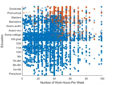
The colors in the scatter plot indicate that, in general, the neural network predicts that people with lower levels of education (12th grade or below) have salaries less than or equal to $50,000 per year. The transparency of some of the points in the lower right of the plot indicates that the model is less confident in this prediction for people who work many hours per week (60 hours or more).

Matlabsolutions.com provides guaranteed satisfaction with a commitment to complete the work within time. Combined with our meticulous work ethics and extensive domain experience, We are the ideal partner for all your homework/assignment needs. We pledge to provide 24*7 support to dissolve all your academic doubts. We are composed of 300+ esteemed Matlab and other experts who have been empanelled after extensive research and quality check.

Matlabsolutions.com provides undivided attention to each Matlab assignment order with a methodical approach to solution. Our network span is not restricted to US, UK and Australia rather extends to countries like Singapore, Canada and UAE. Our Matlab assignment help services include Image Processing Assignments, Electrical Engineering Assignments, Matlab homework help, Matlab Research Paper help, Matlab Simulink help. Get your work done at the best price in industry.