Fit Model to Data
Create a fitted model using fitglm or stepwiseglm. Choose between them as in Choose Fitting Method and Model. For generalized linear models other than those with a normal distribution, give a Distribution name-value pair as in Choose Generalized Linear Model and Link Function. For example,
mdl = fitglm(X,y,'linear','Distribution','poisson')
% or
mdl = fitglm(X,y,'quadratic',...
         'Distribution','binomial')
Examine Quality and Adjust the Fitted Model
After fitting a model, examine the result.
-
Model Display
-
Diagnostic Plots
-
Residuals — Model Quality for Training Data
-
Plots to Understand Predictor Effects and How to Modify a Model
Model Display
A linear regression model shows several diagnostics when you enter its name or enter disp(mdl). This display gives some of the basic information to check whether the fitted model represents the data adequately.
For example, fit a Poisson model to data constructed with two out of five predictors not affecting the response, and with no intercept term:
rng('default') % for reproducibility
X = randn(100,5);
mu = exp(X(:,[1 4 5])*[.4;.2;.3]);
y = poissrnd(mu);
mdl = fitglm(X,y,...
    'linear','Distribution','poisson')
mdl =


Generalized Linear regression model:
    log(y) ~ 1 + x1 + x2 + x3 + x4 + x5
    Distribution = Poisson

Estimated Coefficients:
                   Estimate     SE          tStat       pValue
    (Intercept)     0.039829     0.10793     0.36901       0.71212
    x1               0.38551    0.076116      5.0647    4.0895e-07
    x2             -0.034905    0.086685    -0.40266        0.6872
    x3              -0.17826    0.093552     -1.9054      0.056722
    x4               0.21929     0.09357      2.3436      0.019097
    x5               0.28918      0.1094      2.6432     0.0082126


100 observations, 94 error degrees of freedom
Dispersion: 1
Chi^2-statistic vs. constant model: 44.9, p-value = 1.55e-08
Notice that:
-
The display contains the estimated values of each coefficient in the
Estimatecolumn. These values are reasonably near the true values[0;.4;0;0;.2;.3], except possibly the coefficient ofx3is not terribly near0. -
There is a standard error column for the coefficient estimates.
-
The reported
pValue(which are derived from the t statistics under the assumption of normal errors) for predictors 1, 4, and 5 are small. These are the three predictors that were used to create the response datay. -
The
pValuefor(Intercept),x2andx3are larger than 0.01. These three predictors were not used to create the response datay. ThepValueforx3is just over.05, so might be regarded as possibly significant. -
The display contains the Chi-square statistic.
Diagnostic Plots
Diagnostic plots help you identify outliers, and see other problems in your model or fit. To illustrate these plots, consider binomial regression with a logistic link function.
The logistic model is useful for proportion data. It defines the relationship between the proportion p and the weight w by:
log[p/(1 – p)] = b1 + b2w
This example fits a binomial model to data. The data are derived from carbig.mat, which contains measurements of large cars of various weights. Each weight in w has a corresponding number of cars in total and a corresponding number of poor-mileage cars in poor.
It is reasonable to assume that the values of poor follow binomial distributions, with the number of trials given by total and the percentage of successes depending on w. This distribution can be accounted for in the context of a logistic model by using a generalized linear model with link function log(µ/(1 – µ)) = Xb. This link function is called 'logit'.
w = [2100 2300 2500 2700 2900 3100 ...
     3300 3500 3700 3900 4100 4300]';
total = [48 42 31 34 31 21 23 23 21 16 17 21]';
poor = [1 2 0 3 8 8 14 17 19 15 17 21]';
mdl = fitglm(w,[poor total],...
    'linear','Distribution','binomial','link','logit')
mdl =

Generalized Linear regression model:
    logit(y) ~ 1 + x1
    Distribution = Binomial

Estimated Coefficients:
                   Estimate     SE            tStat      pValue
    (Intercept)       -13.38         1.394    -9.5986    8.1019e-22
    x1             0.0041812    0.00044258     9.4474    3.4739e-21

12 observations, 10 error degrees of freedom
Dispersion: 1
Chi^2-statistic vs. constant model: 242, p-value = 1.3e-54
See how well the model fits the data.
plotSlice(mdl)
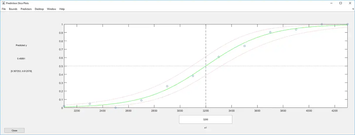
The fit looks reasonably good, with fairly wide confidence bounds.
To examine further details, create a leverage plot.
plotDiagnostics(mdl)

This is typical of a regression with points ordered by the predictor variable. The leverage of each point on the fit is higher for points with relatively extreme predictor values (in either direction) and low for points with average predictor values. In examples with multiple predictors and with points not ordered by predictor value, this plot can help you identify which observations have high leverage because they are outliers as measured by their predictor values.
Residuals — Model Quality for Training Data
There are several residual plots to help you discover errors, outliers, or correlations in the model or data. The simplest residual plots are the default histogram plot, which shows the range of the residuals and their frequencies, and the probability plot, which shows how the distribution of the residuals compares to a normal distribution with matched variance.
This example shows residual plots for a fitted Poisson model. The data construction has two out of five predictors not affecting the response, and no intercept term:
rng('default') % for reproducibility
X = randn(100,5);
mu = exp(X(:,[1 4 5])*[2;1;.5]);
y = poissrnd(mu);
mdl = fitglm(X,y,...
    'linear','Distribution','poisson');
Examine the residuals:
plotResiduals(mdl)
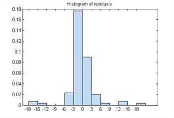
While most residuals cluster near 0, there are several near ±18. So examine a different residuals plot.
plotResiduals(mdl,'fitted')
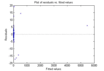
The large residuals don’t seem to have much to do with the sizes of the fitted values.
Perhaps a probability plot is more informative.
plotResiduals(mdl,'probability')
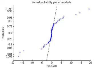
Now it is clear. The residuals do not follow a normal distribution. Instead, they have fatter tails, much as an underlying Poisson distribution.
Plots to Understand Predictor Effects and How to Modify a Model
This example shows how to understand the effect each predictor has on a regression model, and how to modify the model to remove unnecessary terms.
-
Create a model from some predictors in artificial data. The data do not use the second and third columns in
X. So you expect the model not to show much dependence on those predictors.rng('default') % for reproducibility X = randn(100,5); mu = exp(X(:,[1 4 5])*[2;1;.5]); y = poissrnd(mu); mdl = fitglm(X,y,... 'linear','Distribution','poisson'); -
Examine a slice plot of the responses. This displays the effect of each predictor separately.
plotSlice(mdl)
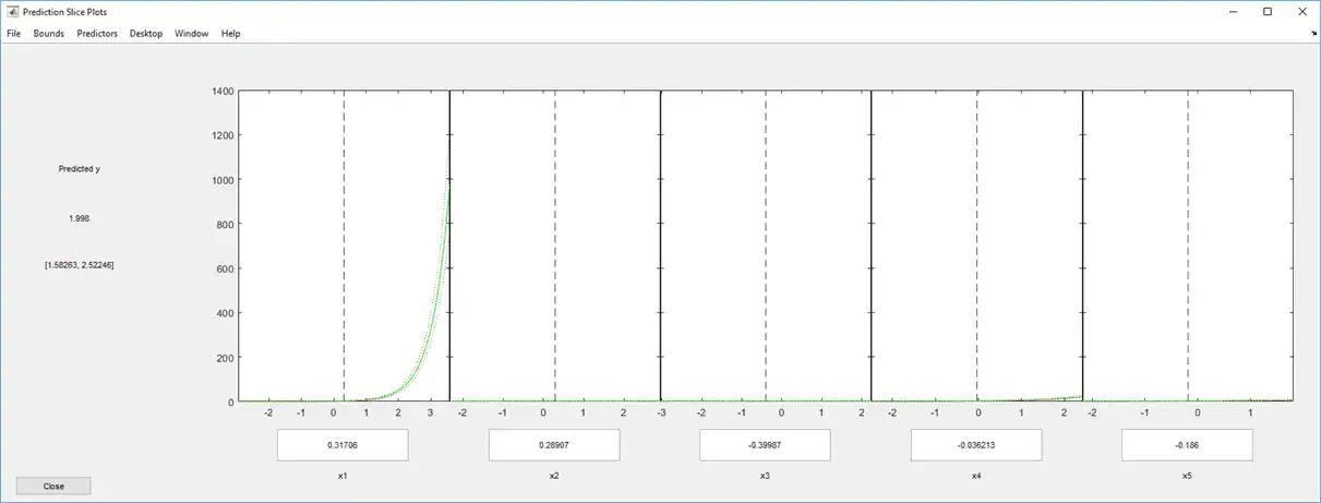
The scale of the first predictor is overwhelming the plot. Disable it using the Predictors menu.


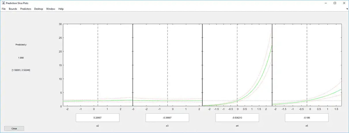
Now it is clear that predictors 2 and 3 have little to no effect.
You can drag the individual predictor values, which are represented by dashed blue vertical lines. You can also choose between simultaneous and non-simultaneous confidence bounds, which are represented by dashed red curves. Dragging the predictor lines confirms that predictors 2 and 3 have little to no effect.
-
Remove the unnecessary predictors using either
removeTermsorstep. Usingstepcan be safer, in case there is an unexpected importance to a term that becomes apparent after removing another term. However, sometimesremoveTermscan be effective whenstepdoes not proceed. In this case, the two give identical results.mdl1 = removeTerms(mdl,'x2 + x3')
mdl1 =


Generalized Linear regression model:
    log(y) ~ 1 + x1 + x4 + x5
    Distribution = Poisson

Estimated Coefficients:
                   Estimate    SE          tStat     pValue
    (Intercept)    0.17604     0.062215    2.8295       0.004662
    x1              1.9122     0.024638    77.614              0
    x4             0.98521     0.026393    37.328    5.6696e-305
    x5             0.61321     0.038435    15.955     2.6473e-57


100 observations, 96 error degrees of freedom
Dispersion: 1
Chi^2-statistic vs. constant model: 4.97e+04, p-value = 0
mdl1 = step(mdl,'NSteps',5,'Upper','linear')
1. Removing x3, Deviance = 93.856, Chi2Stat = 0.00075551, PValue = 0.97807
2. Removing x2, Deviance = 96.333, Chi2Stat = 2.4769, PValue = 0.11553

mdl1 =


Generalized Linear regression model:
    log(y) ~ 1 + x1 + x4 + x5
    Distribution = Poisson

Estimated Coefficients:
                   Estimate    SE          tStat     pValue
    (Intercept)    0.17604     0.062215    2.8295       0.004662
    x1              1.9122     0.024638    77.614              0
    x4             0.98521     0.026393    37.328    5.6696e-305
    x5             0.61321     0.038435    15.955     2.6473e-57


100 observations, 96 error degrees of freedom
Dispersion: 1
Chi^2-statistic vs. constant model: 4.97e+04, p-value = 0
Predict or Simulate Responses to New Data
There are three ways to use a linear model to predict the response to new data:
-
predict -
feval -
random
predict
The predict method gives a prediction of the mean responses and, if requested, confidence bounds.
This example shows how to predict and obtain confidence intervals on the predictions using the predict method.
-
Create a model from some predictors in artificial data. The data do not use the second and third columns in
X. So you expect the model not to show much dependence on these predictors. Construct the model stepwise to include the relevant predictors automatically.rng('default') % for reproducibility X = randn(100,5); mu = exp(X(:,[1 4 5])*[2;1;.5]); y = poissrnd(mu); mdl = stepwiseglm(X,y,... 'constant','upper','linear','Distribution','poisson');1. Adding x1, Deviance = 2515.02869, Chi2Stat = 47242.9622, PValue = 0 2. Adding x4, Deviance = 328.39679, Chi2Stat = 2186.6319, PValue = 0 3. Adding x5, Deviance = 96.3326, Chi2Stat = 232.0642, PValue = 2.114384e-52
-
Generate some new data, and evaluate the predictions from the data.
Xnew = randn(3,5) + repmat([1 2 3 4 5],[3,1]); % new data [ynew,ynewci] = predict(mdl,Xnew)
ynew = 1.0e+04 * 0.1130 1.7375 3.7471 ynewci = 1.0e+04 * 0.0821 0.1555 1.2167 2.4811 2.8419 4.9407
feval
When you construct a model from a table or dataset array, feval is often more convenient for predicting mean responses than predict. However, feval does not provide confidence bounds.
This example shows how to predict mean responses using the feval method.
-
Create a model from some predictors in artificial data. The data do not use the second and third columns in
X. So you expect the model not to show much dependence on these predictors. Construct the model stepwise to include the relevant predictors automatically.rng('default') % for reproducibility X = randn(100,5); mu = exp(X(:,[1 4 5])*[2;1;.5]); y = poissrnd(mu); X = array2table(X); % create data table y = array2table(y); tbl = [X y]; mdl = stepwiseglm(tbl,... 'constant','upper','linear','Distribution','poisson');1. Adding x1, Deviance = 2515.02869, Chi2Stat = 47242.9622, PValue = 0 2. Adding x4, Deviance = 328.39679, Chi2Stat = 2186.6319, PValue = 0 3. Adding x5, Deviance = 96.3326, Chi2Stat = 232.0642, PValue = 2.114384e-52
-
Generate some new data, and evaluate the predictions from the data.
Xnew = randn(3,5) + repmat([1 2 3 4 5],[3,1]); % new data ynew = feval(mdl,Xnew(:,1),Xnew(:,4),Xnew(:,5)) % only need predictors 1,4,5
ynew = 1.0e+04 * 0.1130 1.7375 3.7471Equivalently,
ynew = feval(mdl,Xnew(:,[1 4 5])) % only need predictors 1,4,5
ynew = 1.0e+04 * 0.1130 1.7375 3.7471
random
The random method generates new random response values for specified predictor values. The distribution of the response values is the distribution used in the model. random calculates the mean of the distribution from the predictors, estimated coefficients, and link function. For distributions such as normal, the model also provides an estimate of the variance of the response. For the binomial and Poisson distributions, the variance of the response is determined by the mean; random does not use a separate “dispersion” estimate.
This example shows how to simulate responses using the random method.
-
Create a model from some predictors in artificial data. The data do not use the second and third columns in
X. So you expect the model not to show much dependence on these predictors. Construct the model stepwise to include the relevant predictors automatically.rng('default') % for reproducibility X = randn(100,5); mu = exp(X(:,[1 4 5])*[2;1;.5]); y = poissrnd(mu); mdl = stepwiseglm(X,y,... 'constant','upper','linear','Distribution','poisson');1. Adding x1, Deviance = 2515.02869, Chi2Stat = 47242.9622, PValue = 0 2. Adding x4, Deviance = 328.39679, Chi2Stat = 2186.6319, PValue = 0 3. Adding x5, Deviance = 96.3326, Chi2Stat = 232.0642, PValue = 2.114384e-52
-
Generate some new data, and evaluate the predictions from the data.
Xnew = randn(3,5) + repmat([1 2 3 4 5],[3,1]); % new data ysim = random(mdl,Xnew)
ysim = 1111 17121 37457The predictions from
randomare Poisson samples, so are integers. -
Evaluate the
randommethod again, the result changes.ysim = random(mdl,Xnew)
ysim = 1175 17320 37126
Share Fitted Models
The model display contains enough information to enable someone else to recreate the model in a theoretical sense. For example,
rng('default') % for reproducibility
X = randn(100,5);
mu = exp(X(:,[1 4 5])*[2;1;.5]);
y = poissrnd(mu);
mdl = stepwiseglm(X,y,...
'constant','upper','linear','Distribution','poisson')
1. Adding x1, Deviance = 2515.02869, Chi2Stat = 47242.9622, PValue = 0
2. Adding x4, Deviance = 328.39679, Chi2Stat = 2186.6319, PValue = 0
3. Adding x5, Deviance = 96.3326, Chi2Stat = 232.0642, PValue = 2.114384e-52
mdl =
Generalized Linear regression model:
log(y) ~ 1 + x1 + x4 + x5
Distribution = Poisson
Estimated Coefficients:
Estimate SE tStat pValue
(Intercept) 0.17604 0.062215 2.8295 0.004662
x1 1.9122 0.024638 77.614 0
x4 0.98521 0.026393 37.328 5.6696e-305
x5 0.61321 0.038435 15.955 2.6473e-57
100 observations, 96 error degrees of freedom
Dispersion: 1
Chi^2-statistic vs. constant model: 4.97e+04, p-value = 0
You can access the model description programmatically, too. For example,
mdl.Coefficients.Estimate
ans =

    0.1760
    1.9122
    0.9852
    0.6132
mdl.Formula
ans =

log(y) ~ 1 + x1 + x4 + x5