Linear Regression 4

plotInteraction(mdl,'Cylinders','Weight','predictions')

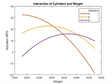
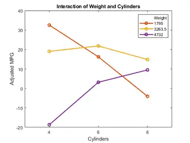
Figure contains an axes object. The axes object with title Interaction of Cylinders and Weight contains 4 objects of type line. These objects represent Cylinders, 4, 6, 8.

Now look at the interactions with various fixed levels of weight.

plotInteraction(mdl,'Weight','Cylinders','predictions')

Figure contains an axes object. The axes object with title Interaction of Weight and Cylinders contains 4 objects of type line. These objects represent Weight, 1795, 3263.5, 4732.

Plots to Understand Terms Effects

This example shows how to understand the effect of each term in a regression model using a variety of available plots.

Create an added variable plot with Weight^2 as the added variable.

plotAdded(mdl,'Weight^2')

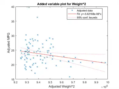
Figure contains an axes object. The axes object with title Added variable plot for Weight^2 contains 3 objects of type line. These objects represent Adjusted data, Fit: y=-5.62168e-06*x, 95% conf. bounds.

This plot shows the results of fitting both Weight^2 and MPG to the terms other than Weight^2. The reason to use plotAdded is to understand what additional improvement in the model you get by adding Weight^2. The coefficient of a line fit to these points is the coefficient of Weight^2 in the full model. The Weight^2 predictor is just over the edge of significance (pValue < 0.05) as you can see in the coefficients table display. You can see that in the plot as well. The confidence bounds look like they could not contain a horizontal line (constant y), so a zero-slope model is not consistent with the data.

Create an added variable plot for the model as a whole.

plotAdded(mdl)

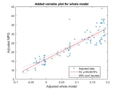
Figure contains an axes object. The axes object with title Added variable plot for whole model contains 3 objects of type line. These objects represent Adjusted data, Fit: y=85.8376*x, 95% conf. bounds.

The model as a whole is very significant, so the bounds don't come close to containing a horizontal line. The slope of the line is the slope of a fit to the predictors projected onto their best-fitting direction, or in other words, the norm of the coefficient vector.

Change Models

There are two ways to change a model:

step — Add or subtract terms one at a time, where step chooses the most important term to add or remove.
addTerms and removeTerms — Add or remove specified terms. Give the terms in any of the forms described in Choose a Model or Range of Models.

If you created a model using stepwiselm, then step can have an effect only if you give different upper or lower models. step does not work when you fit a model using RobustOpts.

For example, start with a linear model of mileage from the carbig data:

load carbig
tbl = table(Acceleration,Displacement,Horsepower,Weight,MPG);
mdl = fitlm(tbl,'linear','ResponseVar','MPG')

mdl = 
Linear regression model:
    MPG ~ 1 + Acceleration + Displacement + Horsepower + Weight

Estimated Coefficients:
                     Estimate         SE         tStat        pValue  
                    __________    __________    ________    __________

    (Intercept)         45.251         2.456      18.424    7.0721e-55
    Acceleration     -0.023148        0.1256     -0.1843       0.85388
    Displacement    -0.0060009     0.0067093    -0.89441       0.37166
    Horsepower       -0.043608      0.016573     -2.6312      0.008849
    Weight          -0.0052805    0.00081085     -6.5123    2.3025e-10


Number of observations: 392, Error degrees of freedom: 387
Root Mean Squared Error: 4.25
R-squared: 0.707,  Adjusted R-Squared: 0.704
F-statistic vs. constant model: 233, p-value = 9.63e-102

Try to improve the model using step for up to 10 steps:

mdl1 = step(mdl,'NSteps',10)

1. Adding Displacement:Horsepower, FStat = 87.4802, pValue = 7.05273e-19

mdl1 = 
Linear regression model:
    MPG ~ 1 + Acceleration + Weight + Displacement*Horsepower

Estimated Coefficients:
                                Estimate         SE         tStat       pValue  
                               __________    __________    _______    __________

    (Intercept)                    61.285        2.8052     21.847    1.8593e-69
    Acceleration                 -0.34401       0.11862       -2.9     0.0039445
    Displacement                -0.081198      0.010071    -8.0623    9.5014e-15
    Horsepower                   -0.24313      0.026068    -9.3265    8.6556e-19
    Weight                     -0.0014367    0.00084041    -1.7095      0.088166
    Displacement:Horsepower    0.00054236    5.7987e-05     9.3531    7.0527e-19


Number of observations: 392, Error degrees of freedom: 386
Root Mean Squared Error: 3.84
R-squared: 0.761,  Adjusted R-Squared: 0.758
F-statistic vs. constant model: 246, p-value = 1.32e-117

step stopped after just one change.

To try to simplify the model, remove the Acceleration and Weight terms from mdl1:

mdl2 = removeTerms(mdl1,'Acceleration + Weight')

mdl2 = 
Linear regression model:
    MPG ~ 1 + Displacement*Horsepower

Estimated Coefficients:
                                Estimate        SE         tStat       pValue   
                               __________    _________    _______    ___________

    (Intercept)                    53.051        1.526     34.765    3.0201e-121
    Displacement                -0.098046    0.0066817    -14.674     4.3203e-39
    Horsepower                   -0.23434     0.019593     -11.96     2.8024e-28
    Displacement:Horsepower    0.00058278    5.193e-05     11.222     1.6816e-25


Number of observations: 392, Error degrees of freedom: 388
Root Mean Squared Error: 3.94
R-squared: 0.747,  Adjusted R-Squared: 0.745
F-statistic vs. constant model: 381, p-value = 3e-115

mdl2 uses just Displacement and Horsepower, and has nearly as good a fit to the data as mdl1 in the Adjusted R-Squared metric.

Predict or Simulate Responses to New Data

A LinearModel object offers three functions to predict or simulate the response to new data: predict, feval, and random.

predict

Use the predict function to predict and obtain confidence intervals on the predictions.

Load the carbig data and create a default linear model of the response MPG to the Acceleration, Displacement, Horsepower, and Weight predictors.

load carbig
X = [Acceleration,Displacement,Horsepower,Weight];
mdl = fitlm(X,MPG);

Create a three-row array of predictors from the minimal, mean, and maximal values. X contains some NaN values, so specify the 'omitnan' option for the mean function. The min and max functions omit NaN values in the calculation by default.

Xnew = [min(X);mean(X,'omitnan');max(X)];

Find the predicted model responses and confidence intervals on the predictions.

[NewMPG, NewMPGCI] = predict(mdl,Xnew)

NewMPG = 3×1

   34.1345
   23.4078
    4.7751

NewMPGCI = 3×2

   31.6115   36.6575
   22.9859   23.8298
    0.6134    8.9367

The confidence bound on the mean response is narrower than those for the minimum or maximum responses.

feval

Use the feval function to predict responses. When you create a model from a table or dataset array, feval is often more convenient than predict for predicting responses. When you have new predictor data, you can pass it to feval without creating a table or matrix. However, feval does not provide confidence bounds.

Load the carbig data set and create a default linear model of the response MPG to the predictors Acceleration, Displacement, Horsepower, and Weight.

load carbig
tbl = table(Acceleration,Displacement,Horsepower,Weight,MPG);
mdl = fitlm(tbl,'linear','ResponseVar','MPG');

Predict the model response for the mean values of the predictors.

NewMPG = feval(mdl,mean(Acceleration,'omitnan'),mean(Displacement,'omitnan'),mean(Horsepower,'omitnan'),mean(Weight,'omitnan'))

NewMPG = 23.4078

random

Use the random function to simulate responses. The random function simulates new random response values, equal to the mean prediction plus a random disturbance with the same variance as the training data.

Load the carbig data and create a default linear model of the response MPG to the Acceleration, Displacement, Horsepower, and Weight predictors.

load carbig
X = [Acceleration,Displacement,Horsepower,Weight];
mdl = fitlm(X,MPG);

Create a three-row array of predictors from the minimal, mean, and maximal values.

Xnew = [min(X);mean(X,'omitnan');max(X)];

Generate new predicted model responses including some randomness.

rng('default') % for reproducibility
NewMPG = random(mdl,Xnew)

NewMPG = 3×1

   36.4178
   31.1958
   -4.8176

Because a negative value of MPG does not seem sensible, try predicting two more times.

NewMPG = random(mdl,Xnew)

NewMPG = 3×1

   37.7959
   24.7615
   -0.7783

NewMPG = random(mdl,Xnew)

NewMPG = 3×1

   32.2931
   24.8628
   19.9715

Clearly, the predictions for the third (maximal) row of Xnew are not reliable.

Share Fitted Models

Suppose you have a linear regression model, such as mdl from the following commands.

load carbig
tbl = table(Acceleration,Displacement,Horsepower,Weight,MPG);
mdl = fitlm(tbl,'linear','ResponseVar','MPG');

To share the model with other people, you can:

Provide the model display.

mdl

mdl = 
Linear regression model:
    MPG ~ 1 + Acceleration + Displacement + Horsepower + Weight

Estimated Coefficients:
                     Estimate         SE         tStat        pValue  
                    __________    __________    ________    __________

    (Intercept)         45.251         2.456      18.424    7.0721e-55
    Acceleration     -0.023148        0.1256     -0.1843       0.85388
    Displacement    -0.0060009     0.0067093    -0.89441       0.37166
    Horsepower       -0.043608      0.016573     -2.6312      0.008849
    Weight          -0.0052805    0.00081085     -6.5123    2.3025e-10


Number of observations: 392, Error degrees of freedom: 387
Root Mean Squared Error: 4.25
R-squared: 0.707,  Adjusted R-Squared: 0.704
F-statistic vs. constant model: 233, p-value = 9.63e-102

Provide the model definition and coefficients.

mdl.Formula

ans = 
MPG ~ 1 + Acceleration + Displacement + Horsepower + Weight

mdl.CoefficientNames

ans = 1x5 cell
  Columns 1 through 4

    {'(Intercept)'}    {'Acceleration'}    {'Displacement'}    {'Horsepower'}

  Column 5

    {'Weight'}

mdl.Coefficients.Estimate

ans = 5×1

   45.2511
   -0.0231
   -0.0060
   -0.0436
   -0.0053

Matlabsolutions.com provides guaranteed satisfaction with a commitment to complete the work within time. Combined with our meticulous work ethics and extensive domain experience, We are the ideal partner for all your homework/assignment needs. We pledge to provide 24*7 support to dissolve all your academic doubts. We are composed of 300+ esteemed Matlab and other experts who have been empanelled after extensive research and quality check.

Matlabsolutions.com provides undivided attention to each Matlab assignment order with a methodical approach to solution. Our network span is not restricted to US, UK and Australia rather extends to countries like Singapore, Canada and UAE. Our Matlab assignment help services include Image Processing Assignments, Electrical Engineering Assignments, Matlab homework help, Matlab Research Paper help, Matlab Simulink help. Get your work done at the best price in industry.