Neural networks

In the MATLAB^® Command Window, load the carbig data set, and create a table containing the different variables.

load carbig
cartable = table(Acceleration,Cylinders,Displacement, ...
    Horsepower,Model_Year,Weight,Origin,MPG);

Click the Apps tab, and then click the Show more arrow on the right to open the apps gallery. In the Machine Learning and Deep Learning group, click Regression Learner.

On the Regression Learner tab, in the File section, click New Session and select From Workspace.

In the New Session from Workspace dialog box, select the table cartable from the Data Set Variable list (if necessary).

As shown in the dialog box, the app selects MPG as the response and the other variables as predictors. For this example, do not change the selections.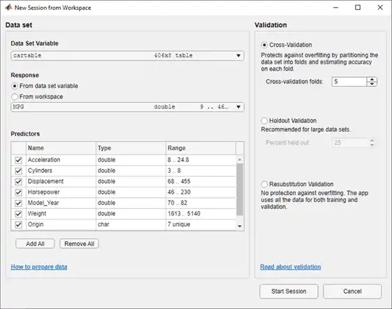

To accept the default validation scheme and continue, click Start Session. The default validation option is 5-fold cross-validation, to protect against overfitting.

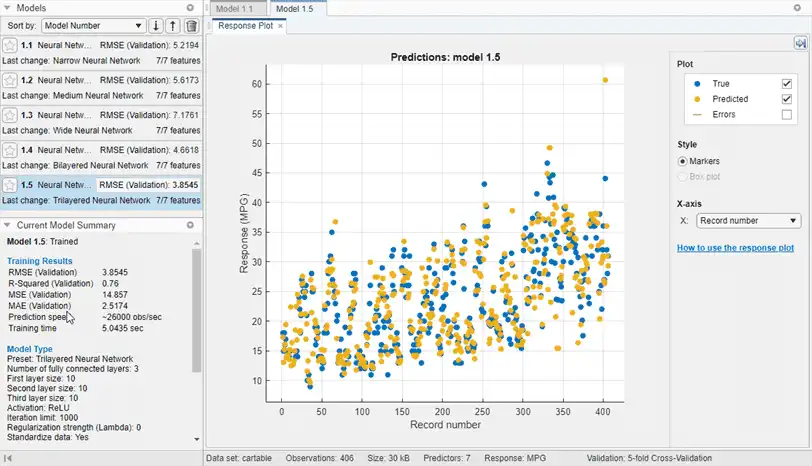
Regression Learner creates a plot of the response with the record number on the x-axis.

Use the response plot to investigate which variables are useful for predicting the response. To visualize the relation between different predictors and the response, select different variables in the X list under X-axis. Note which variables are correlated most clearly with the response.

Create a selection of neural network models. On the Regression Learner tab, in the Model Type section, click the arrow to open the gallery. In the Neural Networks group, click All Neural Networks.

In the Training section, click Train. Regression Learner trains one of each neural network option in the gallery. In the Models pane, the app outlines the RMSE (Validation) (root mean squared error) of the best model.

Select a model in the Models pane to view the results. On the Regression Learner tab, in the Plots section, click the arrow to open the gallery, and then click Response in the Validation Results group. Examine the response plot for the trained model. True responses are in blue, and predicted responses are in yellow.

Under X-axis, select Horsepower and examine the response plot. Both the true and predicted responses are now plotted. Show the prediction errors, drawn as vertical lines between the predicted and true responses, by selecting the Errors check box.

For more information on the currently selected model, consult the Current Model Summary pane. Check and compare additional model characteristics, such as R-squared (coefficient of determination), MAE (mean absolute error), and prediction speed. To learn more, see View and Compare Model Statistics. In the Current Model Summary pane, you can also find details on the currently selected model type, such as options used for training the model.

Plot the predicted response versus the true response. On the Regression Learner tab, in the Plots section, click the arrow to open the gallery, and then click Predicted vs. Actual (Validation) in the Validation Results group. Use this plot to determine how well the regression model makes predictions for different response values.

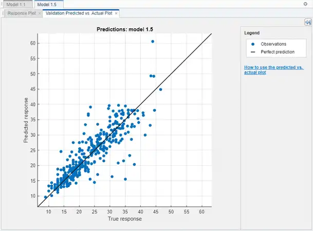
A perfect regression model has predicted responses equal to the true responses, so all the points lie on a diagonal line. The vertical distance from the line to any point is the error of the prediction for that point. A good model has small errors, so the predictions are scattered near the line. Typically, a good model has points scattered roughly symmetrically around the diagonal line. If you can see any clear patterns in the plot, you can most likely improve your model.

Select the other models in the Models pane, open the predicted versus actual plot for each of the models, and then compare the results. See Compare Model Plots by Changing Layout.

In the Model Type gallery, select All Neural Networks again. To try to improve the models, include different features. See if you can improve the models by removing features with low predictive power. On the Regression Learner tab, in the Features section, click Feature Selection.

In the Feature Selection dialog box, clear the check boxes for Acceleration and Cylinders to exclude them from the predictors, and then click OK.

In the Training section, click Train to train the neural network models using the new predictor settings.

Observe the new models in the Models pane. These models are the same neural network models as before, but trained using only five of the seven predictors. For each model, the app displays how many predictors are used. To check which predictors are used, click a model in the Models pane and consult the Feature Selection section of the Current Model Summary pane.

The models with the two features removed perform comparably to the models with all predictors. The models predict no better using all the predictors compared to using only a subset of them. If data collection is expensive or difficult, you might prefer a model that performs satisfactorily without some predictors.

Select the best model in the Models pane and view the residuals plot. On the Regression Learner tab, in the Plots section, click the arrow to open the gallery, and then click Residuals (Validation) in the Validation Results group. The residuals plot displays the difference between the predicted and true responses. To display the residuals as a line graph, in the Style section, choose Lines.

Under X-axis, select the variable to plot on the x-axis. Choose the true response, predicted response, record number, or one of your predictors.

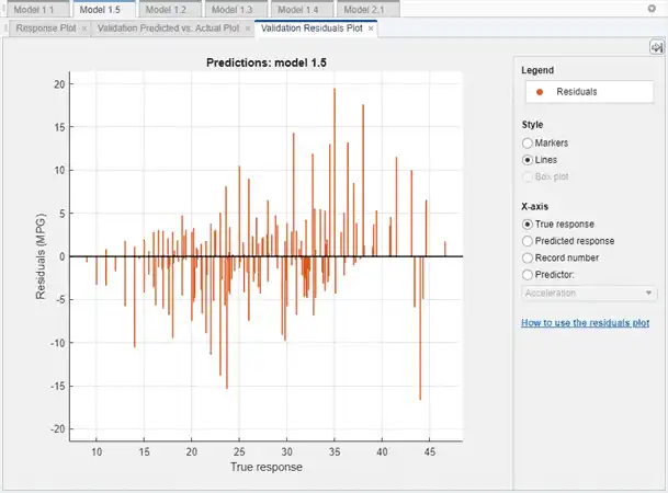
Typically, a good model has residuals scattered roughly symmetrically around 0. If you can see any clear patterns in the residuals, you can most likely improve your model.

You can try to further improve the best model in the Models pane by changing its advanced settings. On the Regression Learner tab, in the Model Type section, click Advanced and select Advanced. Try changing some of the settings, like the sizes of the fully connected layers or the regularization strength, and clicking OK. Then train the new model by clicking Train.

To learn more about neural network model settings, see Neural Networks.

You can export a full or compact version of the trained model to the workspace. On the Regression Learner tab, in the Export section, click Export Model and select either Export Model or Export Compact Model. See Export Regression Model to Predict New Data.

To examine the code for training this model, click Generate Function in the Export section.

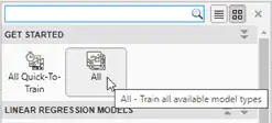
On Regression Learner tab, in the Model Type section, click the arrow to open the gallery of regression models.

In the Get Started group, click All. Then, in the Training section, click Train.