Nonlinear Regression 2

Examine Quality and Adjust the Fitted Nonlinear Model

There are diagnostic plots to help you examine the quality of a model. plotDiagnostics(mdl) gives a variety of plots, including leverage and Cook's distance plots. plotResiduals(mdl) gives the difference between the fitted model and the data.

There are also properties of mdl that relate to the model quality. mdl.RMSE gives the root mean square error between the data and the fitted model. mdl.Residuals.Raw gives the raw residuals. mdl.Diagnostics contains several fields, such as Leverage and CooksDistance, that can help you identify particularly interesting observations.

This example shows how to examine a fitted nonlinear model using diagnostic, residual, and slice plots.

Load the sample data.

load reaction

Create a nonlinear model of rate as a function of reactants using the hougen.m function.

beta0 = ones(5,1);
mdl = fitnlm(reactants,...
    rate,@hougen,beta0);

Make a leverage plot of the data and model.

plotDiagnostics(mdl)

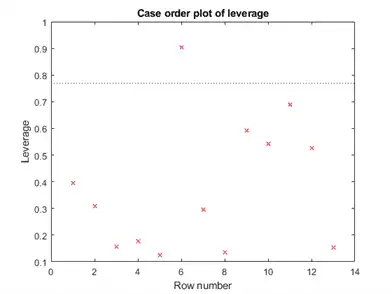
There is one point that has high leverage. Locate the point.

[~,maxl] = max(mdl.Diagnostics.Leverage)

maxl = 6

Examine a residuals plot.

plotResiduals(mdl,'fitted')

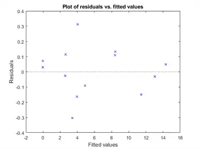
Nothing stands out as an outlier.

Use a slice plot to show the effect of each predictor on the model.

plotSlice(mdl)

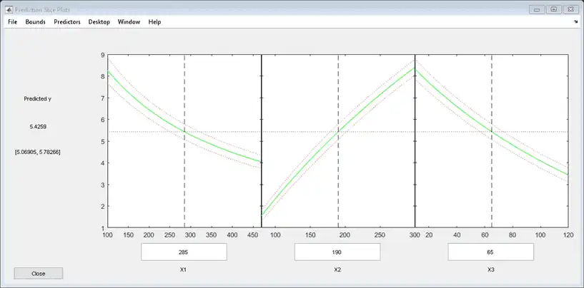
You can drag the vertical dashed blue lines to see the effect of a change in one predictor on the response. For example, drag the X2 line to the right, and notice that the slope of the X3 line changes.

Predict or Simulate Responses Using a Nonlinear Model

This example shows how to use the methods predict, feval, and random to predict and simulate responses to new data.

Randomly generate a sample from a Cauchy distribution.

rng('default')
X = rand(100,1);
X = tan(pi*X - pi/2);

Generate the response according to the model y = b1*(pi /2 + atan((x - b2) / b3)) and add noise to the response.

modelfun = @(b,x) b(1) * ...
    (pi/2 + atan((x - b(2))/b(3)));
y = modelfun([12 5 10],X) + randn(100,1);

Fit a model starting from the arbitrary parameters b = [1,1,1].

beta0 = [1 1 1]; % An arbitrary guess
mdl = fitnlm(X,y,modelfun,beta0)

mdl = 
Nonlinear regression model:
    y ~ b1*(pi/2 + atan((x - b2)/b3))

Estimated Coefficients:
          Estimate      SE       tStat       pValue  
          ________    _______    ______    __________

    b1     12.082     0.80028    15.097    3.3151e-27
    b2     5.0603      1.0825    4.6747    9.5063e-06
    b3       9.64     0.46499    20.732    2.0382e-37


Number of observations: 100, Error degrees of freedom: 97
Root Mean Squared Error: 1.02
R-Squared: 0.92,  Adjusted R-Squared 0.918
F-statistic vs. zero model: 6.45e+03, p-value = 1.72e-111

The fitted values are within a few percent of the parameters [12,5,10].

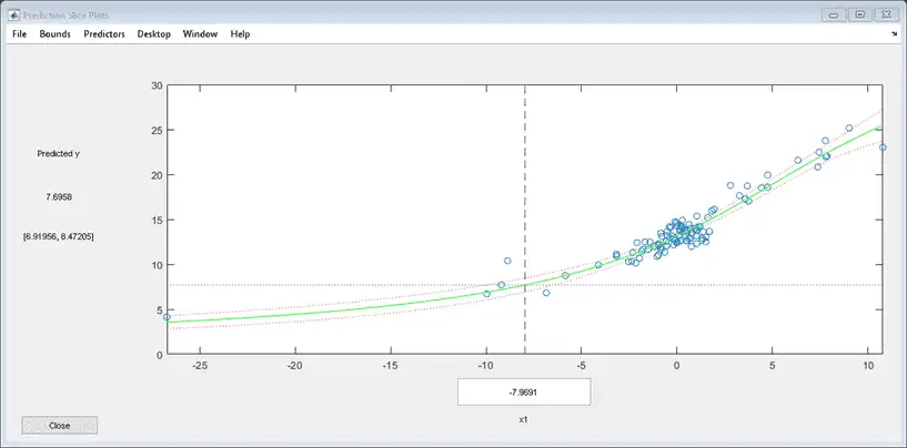
Examine the fit.

plotSlice(mdl)

Xnew = [-15;5;12];
[ynew,ynewci] = predict(mdl,Xnew)

ynew = 3×1

    5.4122
   18.9022
   26.5161

ynewci = 3×2

    4.8233    6.0010
   18.4555   19.3490
   25.0170   28.0151

ds = dataset({X,'X'},{y,'y'});
mdl2 = fitnlm(ds,modelfun,beta0);

Xnew = [-15;5;12];
ynew = feval(mdl2,Xnew)

ynew = 3×1

    5.4122
   18.9022
   26.5161

Xnew = [-15;5;12];
ysim = random(mdl,Xnew)

ysim = 3×1

    6.0505
   19.0893
   25.4647

ysim = random(mdl,Xnew)

ysim = 3×1

    6.3813
   19.2157
   26.6541