Support Vector Machines for Binary Classification 4

Optimize Classifier Fit Using Bayesian Optimization

This example shows how to optimize an SVM classification using the fitcsvm function and the OptimizeHyperparameters name-value argument.

Generate Data

The classification works on locations of points from a Gaussian mixture model. In The Elements of Statistical Learning, Hastie, Tibshirani, and Friedman (2009), page 17 describes the model. The model begins with generating 10 base points for a "green" class, distributed as 2-D independent normals with mean (1,0) and unit variance. It also generates 10 base points for a "red" class, distributed as 2-D independent normals with mean (0,1) and unit variance. For each class (green and red), generate 100 random points as follows:

Choose a base point m of the appropriate color uniformly at random.
Generate an independent random point with 2-D normal distribution with mean m and variance I/5, where I is the 2-by-2 identity matrix. In this example, use a variance I/50 to show the advantage of optimization more clearly.

Generate the 10 base points for each class.

rng('default') % For reproducibility
grnpop = mvnrnd([1,0],eye(2),10);
redpop = mvnrnd([0,1],eye(2),10);

View the base points.

plot(grnpop(:,1),grnpop(:,2),'go')
hold on
plot(redpop(:,1),redpop(:,2),'ro')
hold off

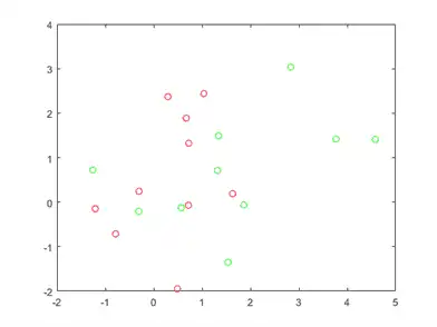
Figure contains an axes object. The axes object contains 2 objects of type line.

Since some red base points are close to green base points, it can be difficult to classify the data points based on location alone.

Generate the 100 data points of each class.

redpts = zeros(100,2);
grnpts = redpts;
for i = 1:100
    grnpts(i,:) = mvnrnd(grnpop(randi(10),:),eye(2)*0.02);
    redpts(i,:) = mvnrnd(redpop(randi(10),:),eye(2)*0.02);
end

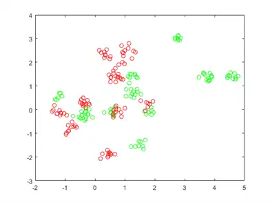
View the data points.

figure
plot(grnpts(:,1),grnpts(:,2),'go')
hold on
plot(redpts(:,1),redpts(:,2),'ro')
hold off

Figure contains an axes object. The axes object contains 2 objects of type line.

Prepare Data for Classification

Put the data into one matrix, and make a vector grp that labels the class of each point. 1 indicates the green class, and –1 indicates the red class.

cdata = [grnpts;redpts];
grp = ones(200,1);
grp(101:200) = -1;

Prepare Cross-Validation

Set up a partition for cross-validation.

c = cvpartition(200,'KFold',10);

This step is optional. If you specify a partition for the optimization, then you can compute an actual cross-validation loss for the returned model.

Optimize Fit

To find a good fit, meaning one with optimal hyperparameters that minimize the cross-validation loss, use Bayesian optimization. Specify a list of hyperparameters to optimize by using the OptimizeHyperparameters name-value argument, and specify optimization options by using the HyperparameterOptimizationOptions name-value argument.

Specify 'OptimizeHyperparameters' as 'auto'. The 'auto' option includes a typical set of hyperparameters to optimize. fitcsvm finds optimal values of BoxConstraint and KernelScale. Set the hyperparameter optimization options to use the cross-validation partition c and to choose the 'expected-improvement-plus' acquisition function for reproducibility. The default acquisition function depends on run time and, therefore, can give varying results.

opts = struct('CVPartition',c,'AcquisitionFunctionName','expected-improvement-plus');
Mdl = fitcsvm(cdata,grp,'KernelFunction','rbf', ...
    'OptimizeHyperparameters','auto','HyperparameterOptimizationOptions',opts)

|=====================================================================================================|
| Iter | Eval   | Objective   | Objective   | BestSoFar   | BestSoFar   | BoxConstraint|  KernelScale |
|      | result |             | runtime     | (observed)  | (estim.)    |              |              |
|=====================================================================================================|
|    1 | Best   |       0.345 |     0.29522 |       0.345 |       0.345 |      0.00474 |       306.44 |
|    2 | Best   |       0.115 |     0.18714 |       0.115 |     0.12678 |       430.31 |       1.4864 |
|    3 | Accept |        0.52 |     0.27751 |       0.115 |      0.1152 |     0.028415 |     0.014369 |
|    4 | Accept |        0.61 |       0.297 |       0.115 |     0.11504 |       133.94 |    0.0031427 |
|    5 | Accept |        0.34 |     0.40509 |       0.115 |     0.11504 |     0.010993 |       5.7742 |
|    6 | Best   |       0.085 |      0.2515 |       0.085 |    0.085039 |       885.63 |      0.68403 |
|    7 | Accept |       0.105 |     0.25066 |       0.085 |    0.085428 |       0.3057 |      0.58118 |
|    8 | Accept |        0.21 |     0.26477 |       0.085 |     0.09566 |      0.16044 |      0.91824 |
|    9 | Accept |       0.085 |     0.23688 |       0.085 |     0.08725 |       972.19 |      0.46259 |
|   10 | Accept |         0.1 |     0.42455 |       0.085 |    0.090952 |       990.29 |        0.491 |
|   11 | Best   |        0.08 |     0.35181 |        0.08 |    0.079362 |       2.5195 |        0.291 |
|   12 | Accept |        0.09 |      0.2114 |        0.08 |     0.08402 |       14.338 |      0.44386 |
|   13 | Accept |         0.1 |     0.20009 |        0.08 |     0.08508 |    0.0022577 |      0.23803 |
|   14 | Accept |        0.11 |     0.49489 |        0.08 |    0.087378 |       0.2115 |      0.32109 |
|   15 | Best   |        0.07 |     0.29763 |        0.07 |    0.081507 |        910.2 |      0.25218 |
|   16 | Best   |       0.065 |     0.36104 |       0.065 |    0.072457 |       953.22 |      0.26253 |
|   17 | Accept |       0.075 |     0.38855 |       0.065 |    0.072554 |       998.74 |      0.23087 |
|   18 | Accept |       0.295 |     0.27085 |       0.065 |    0.072647 |       996.18 |       44.626 |
|   19 | Accept |        0.07 |     0.31933 |       0.065 |     0.06946 |       985.37 |      0.27389 |
|   20 | Accept |       0.165 |     0.27464 |       0.065 |    0.071622 |     0.065103 |      0.13679 |
|=====================================================================================================|
| Iter | Eval   | Objective   | Objective   | BestSoFar   | BestSoFar   | BoxConstraint|  KernelScale |
|      | result |             | runtime     | (observed)  | (estim.)    |              |              |
|=====================================================================================================|
|   21 | Accept |       0.345 |     0.30824 |       0.065 |    0.071764 |        971.7 |       999.01 |
|   22 | Accept |        0.61 |     0.26964 |       0.065 |    0.071967 |    0.0010168 |    0.0010005 |
|   23 | Accept |       0.345 |     0.34764 |       0.065 |    0.071959 |    0.0011459 |       995.89 |
|   24 | Accept |        0.35 |     0.22277 |       0.065 |    0.071863 |    0.0010003 |       40.628 |
|   25 | Accept |        0.24 |     0.46237 |       0.065 |    0.072124 |       996.55 |       10.423 |
|   26 | Accept |        0.61 |     0.48664 |       0.065 |    0.072067 |       994.71 |    0.0010063 |
|   27 | Accept |        0.47 |     0.20158 |       0.065 |     0.07218 |       993.69 |     0.029723 |
|   28 | Accept |         0.3 |     0.17353 |       0.065 |    0.072291 |       993.15 |       170.01 |
|   29 | Accept |        0.16 |     0.41714 |       0.065 |    0.072103 |       992.81 |       3.8594 |
|   30 | Accept |       0.365 |     0.42269 |       0.065 |    0.072112 |    0.0010017 |     0.044287 |

Figure contains an axes object. The axes object with title Min objective vs. Number of function evaluations contains 2 objects of type line. These objects represent Min observed objective, Estimated min objective.

Figure contains an axes object. The axes object with title Objective function model contains 5 objects of type line, surface, contour. These objects represent Observed points, Model mean, Next point, Model minimum feasible.

__________________________________________________________
Optimization completed.
MaxObjectiveEvaluations of 30 reached.
Total function evaluations: 30
Total elapsed time: 42.6693 seconds
Total objective function evaluation time: 9.3728

Best observed feasible point:
    BoxConstraint    KernelScale
    _____________    ___________

       953.22          0.26253  

Observed objective function value = 0.065
Estimated objective function value = 0.073726
Function evaluation time = 0.36104

Best estimated feasible point (according to models):
    BoxConstraint    KernelScale
    _____________    ___________

       985.37          0.27389  

Estimated objective function value = 0.072112
Estimated function evaluation time = 0.29981

Mdl = 
  ClassificationSVM
                         ResponseName: 'Y'
                CategoricalPredictors: []
                           ClassNames: [-1 1]
                       ScoreTransform: 'none'
                      NumObservations: 200
    HyperparameterOptimizationResults: [1x1 BayesianOptimization]
                                Alpha: [77x1 double]
                                 Bias: -0.2352
                     KernelParameters: [1x1 struct]
                       BoxConstraints: [200x1 double]
                      ConvergenceInfo: [1x1 struct]
                      IsSupportVector: [200x1 logical]
                               Solver: 'SMO'


  Properties, Methods

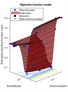
fitcsvm returns a ClassificationSVM model object that uses the best estimated feasible point. The best estimated feasible point is the set of hyperparameters that minimizes the upper confidence bound of the cross-validation loss based on the underlying Gaussian process model of the Bayesian optimization process.

The Bayesian optimization process internally maintains a Gaussian process model of the objective function. The objective function is the cross-validated misclassification rate for classification. For each iteration, the optimization process updates the Gaussian process model and uses the model to find a new set of hyperparameters. Each line of the iterative display shows the new set of hyperparameters and these column values:

Objective — Objective function value computed at the new set of hyperparameters.
Objective runtime — Objective function evaluation time.
Eval result — Result report, specified as Accept, Best, or Error. Accept indicates that the objective function returns a finite value, and Error indicates that the objective function returns a value that is not a finite real scalar. Best indicates that the objective function returns a finite value that is lower than previously computed objective function values.
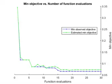
BestSoFar(observed) — The minimum objective function value computed so far. This value is either the objective function value of the current iteration (if the Eval result value for the current iteration is Best) or the value of the previous Best iteration.
BestSoFar(estim.) — At each iteration, the software estimates the upper confidence bounds of the objective function values, using the updated Gaussian process model, at all the sets of hyperparameters tried so far. Then the software chooses the point with the minimum upper confidence bound. The BestSoFar(estim.) value is the objective function value returned by the predictObjective function at the minimum point.

The plot below the iterative display shows the BestSoFar(observed) and BestSoFar(estim.) values in blue and green, respectively.

The returned object Mdl uses the best estimated feasible point, that is, the set of hyperparameters that produces the BestSoFar(estim.) value in the final iteration based on the final Gaussian process model.

You can obtain the best point from the HyperparameterOptimizationResults property or by using the bestPoint function.

Mdl.HyperparameterOptimizationResults.XAtMinEstimatedObjective

ans=1×2 table
    BoxConstraint    KernelScale
    _____________    ___________

       985.37          0.27389

[x,CriterionValue,iteration] = bestPoint(Mdl.HyperparameterOptimizationResults)

x=1×2 table
    BoxConstraint    KernelScale
    _____________    ___________

       985.37          0.27389

CriterionValue = 0.0888

iteration = 19

By default, the bestPoint function uses the 'min-visited-upper-confidence-interval' criterion. This criterion chooses the hyperparameters obtained from the 19th iteration as the best point. CriterionValue is the upper bound of the cross-validated loss computed by the final Gaussian process model. Compute the actual cross-validated loss by using the partition c.

L_MinEstimated = kfoldLoss(fitcsvm(cdata,grp,'CVPartition',c,'KernelFunction','rbf', ...
    'BoxConstraint',x.BoxConstraint,'KernelScale',x.KernelScale))

L_MinEstimated = 0.0700

The actual cross-validated loss is close to the estimated value. The Estimated objective function value is displayed below the plots of the optimization results.

You can also extract the best observed feasible point (that is, the last Best point in the iterative display) from the HyperparameterOptimizationResults property or by specifying Criterion as 'min-observed'.

Mdl.HyperparameterOptimizationResults.XAtMinObjective

ans=1×2 table
    BoxConstraint    KernelScale
    _____________    ___________

       953.22          0.26253

[x_observed,CriterionValue_observed,iteration_observed] = bestPoint(Mdl.HyperparameterOptimizationResults,'Criterion','min-observed')

x_observed=1×2 table
    BoxConstraint    KernelScale
    _____________    ___________

       953.22          0.26253

CriterionValue_observed = 0.0650

iteration_observed = 16

The 'min-observed' criterion chooses the hyperparameters obtained from the 16th iteration as the best point. CriterionValue_observed is the actual cross-validated loss computed using the selected hyperparameters. For more information, see the Criterion name-value argument of bestPoint.

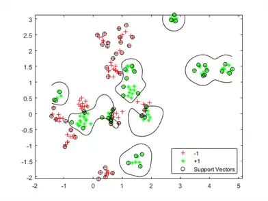
Visualize the optimized classifier.

d = 0.02;
[x1Grid,x2Grid] = meshgrid(min(cdata(:,1)):d:max(cdata(:,1)), ...
    min(cdata(:,2)):d:max(cdata(:,2)));
xGrid = [x1Grid(:),x2Grid(:)];
[~,scores] = predict(Mdl,xGrid);

figure
h(1:2) = gscatter(cdata(:,1),cdata(:,2),grp,'rg','+*');
hold on
h(3) = plot(cdata(Mdl.IsSupportVector,1), ...
    cdata(Mdl.IsSupportVector,2),'ko');
contour(x1Grid,x2Grid,reshape(scores(:,2),size(x1Grid)),[0 0],'k');
legend(h,{'-1','+1','Support Vectors'},'Location','Southeast');

Figure contains an axes object. The axes object contains 4 objects of type line, contour. These objects represent -1, +1, Support Vectors.

Evaluate Accuracy on New Data

Generate and classify new test data points.

grnobj = gmdistribution(grnpop,.2*eye(2));
redobj = gmdistribution(redpop,.2*eye(2));

newData = random(grnobj,10);
newData = [newData;random(redobj,10)];
grpData = ones(20,1); % green = 1
grpData(11:20) = -1; % red = -1

v = predict(Mdl,newData);

Compute the misclassification rates on the test data set.

L_Test = loss(Mdl,newData,grpData)

L_Test = 0.3500

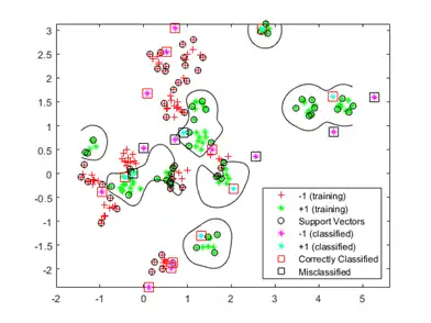
Determine which new data points are classified correctly. Format the correctly classified points in red squares and the incorrectly classified points in black squares.

h(4:5) = gscatter(newData(:,1),newData(:,2),v,'mc','**');

mydiff = (v == grpData); % Classified correctly

for ii = mydiff % Plot red squares around correct pts
    h(6) = plot(newData(ii,1),newData(ii,2),'rs','MarkerSize',12);
end

for ii = not(mydiff) % Plot black squares around incorrect pts
    h(7) = plot(newData(ii,1),newData(ii,2),'ks','MarkerSize',12);
end
legend(h,{'-1 (training)','+1 (training)','Support Vectors', ...
    '-1 (classified)','+1 (classified)', ...
    'Correctly Classified','Misclassified'}, ...
    'Location','Southeast');
hold off

Figure contains an axes object. The axes object contains 8 objects of type line, contour. These objects represent -1 (training), +1 (training), Support Vectors, -1 (classified), +1 (classified), Correctly Classified, Misclassified.

More Page 5

Matlabsolutions.com provides guaranteed satisfaction with a commitment to complete the work within time. Combined with our meticulous work ethics and extensive domain experience, We are the ideal partner for all your homework/assignment needs. We pledge to provide 24*7 support to dissolve all your academic doubts. We are composed of 300+ esteemed Matlab and other experts who have been empanelled after extensive research and quality check.

Matlabsolutions.com provides undivided attention to each Matlab assignment order with a methodical approach to solution. Our network span is not restricted to US, UK and Australia rather extends to countries like Singapore, Canada and UAE. Our Matlab assignment help services include Image Processing Assignments, Electrical Engineering Assignments, Matlab homework help, Matlab Research Paper help, Matlab Simulink help. Get your work done at the best price in industry.