Plot Posterior Probability Regions for SVM Classification Models
This example shows how to predict posterior probabilities of SVM models over a grid of observations, and then plot the posterior probabilities over the grid. Plotting posterior probabilities exposes decision boundaries.
Load Fisher's iris data set. Train the classifier using the petal lengths and widths, and remove the virginica species from the data.
load fisheriris
classKeep = ~strcmp(species,'virginica');
X = meas(classKeep,3:4);
y = species(classKeep);
Train an SVM classifier using the data. It is good practice to specify the order of the classes.
SVMModel = fitcsvm(X,y,'ClassNames',{'setosa','versicolor'});
Estimate the optimal score transformation function.
rng(1); % For reproducibility
[SVMModel,ScoreParameters] = fitPosterior(SVMModel);
Warning: Classes are perfectly separated. The optimal score-to-posterior transformation is a step function.
ScoreParameters
ScoreParameters = struct with fields:
                        Type: 'step'
                  LowerBound: -0.8431
                  UpperBound: 0.6897
    PositiveClassProbability: 0.5000
The optimal score transformation function is the step function because the classes are separable. The fields LowerBound and UpperBound of ScoreParameters indicate the lower and upper end points of the interval of scores corresponding to observations within the class-separating hyperplanes (the margin). No training observation falls within the margin. If a new score is in the interval, then the software assigns the corresponding observation a positive class posterior probability, i.e., the value in the PositiveClassProbability field of ScoreParameters.
Define a grid of values in the observed predictor space. Predict the posterior probabilities for each instance in the grid.
xMax = max(X);
xMin = min(X);
d = 0.01;
[x1Grid,x2Grid] = meshgrid(xMin(1):d:xMax(1),xMin(2):d:xMax(2));

[~,PosteriorRegion] = predict(SVMModel,[x1Grid(:),x2Grid(:)]);
Plot the positive class posterior probability region and the training data.
figure;
contourf(x1Grid,x2Grid,...
        reshape(PosteriorRegion(:,2),size(x1Grid,1),size(x1Grid,2)));
h = colorbar;
h.Label.String = 'P({\it{versicolor}})';
h.YLabel.FontSize = 16;
caxis([0 1]);
colormap jet;

hold on
gscatter(X(:,1),X(:,2),y,'mc','.x',[15,10]);
sv = X(SVMModel.IsSupportVector,:);
plot(sv(:,1),sv(:,2),'yo','MarkerSize',15,'LineWidth',2);
axis tight
hold off
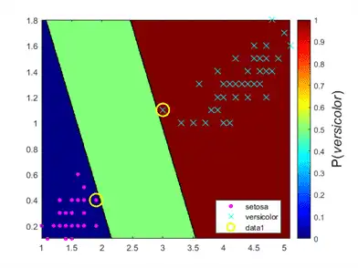
In two-class learning, if the classes are separable, then there are three regions: one where observations have positive class posterior probability 0, one where it is 1, and the other where it is the positive class prior probability.
Analyze Images Using Linear Support Vector Machines
This example shows how to determine which quadrant of an image a shape occupies by training an error-correcting output codes (ECOC) model comprised of linear SVM binary learners. This example also illustrates the disk-space consumption of ECOC models that store support vectors, their labels, and the estimated α coefficients.
Create the Data Set
Randomly place a circle with radius five in a 50-by-50 image. Make 5000 images. Create a label for each image indicating the quadrant that the circle occupies. Quadrant 1 is in the upper right, quadrant 2 is in the upper left, quadrant 3 is in the lower left, and quadrant 4 is in the lower right. The predictors are the intensities of each pixel.
d = 50;  % Height and width of the images in pixels
n = 5e4; % Sample size

X = zeros(n,d^2); % Predictor matrix preallocation
Y = zeros(n,1);   % Label preallocation
theta = 0:(1/d):(2*pi);
r = 5;            % Circle radius
rng(1);           % For reproducibility

for j = 1:n
    figmat = zeros(d);                       % Empty image
    c = datasample((r + 1):(d - r - 1),2);   % Random circle center
    x = r*cos(theta) + c(1);                 % Make the circle
    y = r*sin(theta) + c(2);
    idx = sub2ind([d d],round(y),round(x));  % Convert to linear indexing
    figmat(idx) = 1;                         % Draw the circle
    X(j,:) = figmat(:);                % Store the data
    Y(j) = (c(2) >= floor(d/2)) + 2*(c(2) < floor(d/2)) + ...
        (c(1) < floor(d/2)) + ...
        2*((c(1) >= floor(d/2)) & (c(2) < floor(d/2))); % Determine the quadrant
end
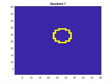
Plot an observation.
figure
imagesc(figmat)
h = gca;
h.YDir = 'normal';
title(sprintf('Quadrant %d',Y(end)))
Train the ECOC Model
Use a 25% holdout sample and specify the training and holdout sample indices.
p = 0.25;
CVP = cvpartition(Y,'Holdout',p); % Cross-validation data partition
isIdx = training(CVP);            % Training sample indices
oosIdx = test(CVP);               % Test sample indices
Create an SVM template that specifies storing the support vectors of the binary learners. Pass it and the training data to fitcecoc to train the model. Determine the training sample classification error.
t = templateSVM('SaveSupportVectors',true);
MdlSV = fitcecoc(X(isIdx,:),Y(isIdx),'Learners',t);
isLoss = resubLoss(MdlSV)
isLoss = 0
MdlSV is a trained ClassificationECOC multiclass model. It stores the training data and the support vectors of each binary learner. For large data sets, such as those in image analysis, the model can consume a lot of memory.
Determine the amount of disk space that the ECOC model consumes.
infoMdlSV = whos('MdlSV');
mbMdlSV = infoMdlSV.bytes/1.049e6
mbMdlSV = 763.6150
The model consumes 763.6 MB.
Improve Model Efficiency
You can assess out-of-sample performance. You can also assess whether the model has been overfit with a compacted model that does not contain the support vectors, their related parameters, and the training data.
Discard the support vectors and related parameters from the trained ECOC model. Then, discard the training data from the resulting model by using compact.
Mdl = discardSupportVectors(MdlSV);
CMdl = compact(Mdl);
info = whos('Mdl','CMdl');
[bytesCMdl,bytesMdl] = info.bytes;
memReduction = 1 - [bytesMdl bytesCMdl]/infoMdlSV.bytes
memReduction = 1×2

    0.0626    0.9996
In this case, discarding the support vectors reduces the memory consumption by about 6%. Compacting and discarding support vectors reduces the size by about 99.96%.
An alternative way to manage support vectors is to reduce their numbers during training by specifying a larger box constraint, such as 100. Though SVM models that use fewer support vectors are more desirable and consume less memory, increasing the value of the box constraint tends to increase the training time.
Remove MdlSV and Mdl from the workspace.
clear Mdl MdlSV
Assess Holdout Sample Performance
Calculate the classification error of the holdout sample. Plot a sample of the holdout sample predictions.
oosLoss = loss(CMdl,X(oosIdx,:),Y(oosIdx))
oosLoss = 0
yHat = predict(CMdl,X(oosIdx,:));
nVec = 1:size(X,1);
oosIdx = nVec(oosIdx);

figure;
for j = 1:9
    subplot(3,3,j)
    imagesc(reshape(X(oosIdx(j),:),[d d]))
    h = gca;
    h.YDir = 'normal';
    title(sprintf('Quadrant: %d',yHat(j)))
end
text(-1.33*d,4.5*d + 1,'Predictions','FontSize',17)
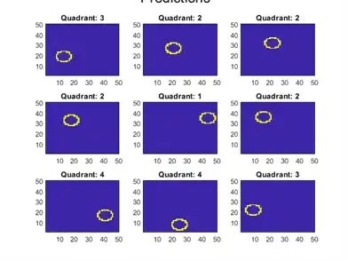
The model does not misclassify any holdout sample observations.