Train Generalized Additive Model for Binary Classification 2

Assess Predictive Performance on New Observations

Assess the performance of the trained model by using the test sample adulttest and the object functions predict, loss, edge, and margin. You can use a full or compact model with these functions.

If you want to assess the performance of the training data set, use the resubstitution object functions: resubPredict, resubLoss, resubMargin, and resubEdge. To use these functions, you must use the full model that contains the training data.

Create a compact model to reduce the size of the trained model.

CMdl = compact(Mdl);
whos('Mdl','CMdl')

  Name      Size              Bytes  Class                                                 Attributes

  CMdl      1x1             5126918  classreg.learning.classif.CompactClassificationGAM              
  Mdl       1x1             5272831  ClassificationGAM                                               

Predict labels and scores for the test data set (adulttest), and compute model statistics (loss, margin, and edge) using the test data set.

[labels,scores] = predict(CMdl,adulttest);
L = loss(CMdl,adulttest,'Weights',adulttest.fnlwgt);
M = margin(CMdl,adulttest);
E = edge(CMdl,adulttest,'Weights',adulttest.fnlwgt);

Predict labels and scores and compute the statistics without including interaction terms in the trained model.

[labels_nointeraction,scores_nointeraction] = predict(CMdl,adulttest,'IncludeInteractions',false);
L_nointeractions = loss(CMdl,adulttest,'Weights',adulttest.fnlwgt,'IncludeInteractions',false);
M_nointeractions = margin(CMdl,adulttest,'IncludeInteractions',false);
E_nointeractions = edge(CMdl,adulttest,'Weights',adulttest.fnlwgt,'IncludeInteractions',false);

Compare the results obtained by including both linear and interaction terms to the results obtained by including only linear terms.

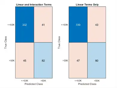
Create a confusion chart from the true labels adulttest.salary and the predicted labels.

tiledlayout(1,2);
nexttile
confusionchart(adulttest.salary,labels)
title('Linear and Interaction Terms')
nexttile
confusionchart(adulttest.salary,labels_nointeraction)
title('Linear Terms Only')

Display the computed loss and edge values.

table([L; E], [L_nointeractions; E_nointeractions], ...
    'VariableNames',{'Linear and Interaction Terms','Only Linear Terms'}, ...
    'RowNames',{'Loss','Edge'})

ans=2×2 table
            Linear and Interaction Terms    Only Linear Terms
            ____________________________    _________________

    Loss               0.1748                    0.17872     
    Edge              0.57902                    0.54756     

The model achieves a smaller loss value and a higher edge value when both linear and interaction terms are included.

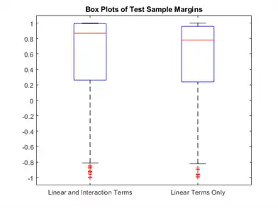
Display the distributions of the margins using box plots.

figure
boxplot([M M_nointeractions],'Labels',{'Linear and Interaction Terms','Linear Terms Only'})
title('Box Plots of Test Sample Margins')

Interpret Prediction

Interpret the prediction for the first test observation by using the plotLocalEffects function. Also, create partial dependence plots for some important terms in the model by using the plotPartialDependence function.

Classify the first observation of the test data, and plot the local effects of the terms in CMdl on the prediction. To display an existing underscore in any predictor name, change the TickLabelInterpreter value of the axes to 'none'.

[label,score] = predict(CMdl,adulttest(1,:))

label = categorical
     <=50K 

score = 1×2

    0.9895    0.0105

f1 = figure;
plotLocalEffects(CMdl,adulttest(1,:))
f1.CurrentAxes.TickLabelInterpreter = 'none';

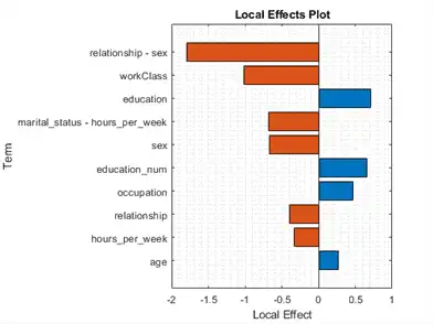
The predict function classifies the first observation adulttest(1,:) as '<=50K'. The plotLocalEffects function creates a horizontal bar graph that shows the local effects of the 10 most important terms on the prediction. Each local effect value shows the contribution of each term to the classification score for '<=50K', which is the logit of the posterior probability that the classification is '<=50K' for the observation.

Create a partial dependence plot for the term age. Specify both the training and test data sets to compute the partial dependence values using both sets.

figure
plotPartialDependence(CMdl,'age',label,[adultdata; adulttest])

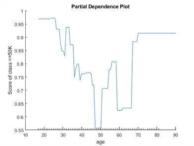
The plotted line represents the averaged partial relationships between the predictor age and the score of the class <=50K in the trained model. The x-axis minor ticks represent the unique values in the predictor age.

Create partial dependence plots for the terms education_num and relationship.

f2 = figure;
plotPartialDependence(CMdl,["education_num","relationship"],label,[adultdata; adulttest])
f2.CurrentAxes.TickLabelInterpreter = 'none';
view([55 40])

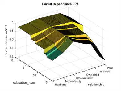
The plot shows the partial dependence of the score value for the class <=50 on education_num and relationship.