Create and Work with Tables

This example shows how to create a table from workspace variables, work with table data, and write tables to files for later use. table is a data type for collecting heterogeneous data and metadata properties such as variable names, row names, descriptions, and variable units, in a single container.

Tables are suitable for column-oriented or tabular data that are often stored as columns in a text file or in a spreadsheet. Each variable in a table can have a different data type, but must have the same number of rows. However, variables in a table are not restricted to column vectors. For example, a table variable can contain a matrix with multiple columns as long as it has the same number of rows as the other table variables. A typical use for a table is to store experimental data, where rows represent different observations and columns represent different measured variables.

Tables are convenient containers for collecting and organizing related data variables and for viewing and summarizing data. For example, you can extract variables to perform calculations and conveniently add the results as new table variables. When you finish your calculations, write the table to a file to save your results.

Create and View Table

Create a table from workspace variables and view it. Alternatively, use the Import Tool or the readtable function to create a table from a spreadsheet or a text file. When you import data from a file using these functions, each column becomes a table variable.

Load sample data for 100 patients from the patients MAT-file to workspace variables.

load patients
whos

  Name                            Size            Bytes  Class      Attributes

  Age                           100x1               800  double               
  Diastolic                     100x1               800  double               
  Gender                        100x1             11412  cell                 
  Height                        100x1               800  double               
  LastName                      100x1             11616  cell                 
  Location                      100x1             14208  cell                 
  SelfAssessedHealthStatus      100x1             11540  cell                 
  Smoker                        100x1               100  logical              
  Systolic                      100x1               800  double               
  Weight                        100x1               800  double

Populate a table with column-oriented variables that contain patient data. You can access and assign table variables by name. When you assign a table variable from a workspace variable, you can assign the table variable a different name.

Create a table and populate it with the Gender, Smoker, Height, and Weight workspace variables. Display the first five rows.

T = table(Gender,Smoker,Height,Weight);
T(1:5,:)

ans=5×4 table
      Gender      Smoker    Height    Weight
    __________    ______    ______    ______

    {'Male'  }    true        71       176  
    {'Male'  }    false       69       163  
    {'Female'}    false       64       131  
    {'Female'}    false       67       133  
    {'Female'}    false       64       119

As an alternative, use the readtable function to read the patient data from a comma-delimited file. readtable reads all the columns that are in a file.

Create a table by reading all columns from the file, patients.dat.

T2 = readtable('patients.dat');
T2(1:5,:)

ans=5×10 table
      LastName        Gender      Age              Location               Height    Weight    Smoker    Systolic    Diastolic    SelfAssessedHealthStatus
    ____________    __________    ___    _____________________________    ______    ______    ______    ________    _________    ________________________

    {'Smith'   }    {'Male'  }    38     {'County General Hospital'  }      71       176        1         124          93             {'Excellent'}      
    {'Johnson' }    {'Male'  }    43     {'VA Hospital'              }      69       163        0         109          77             {'Fair'     }      
    {'Williams'}    {'Female'}    38     {'St. Mary's Medical Center'}      64       131        0         125          83             {'Good'     }      
    {'Jones'   }    {'Female'}    40     {'VA Hospital'              }      67       133        0         117          75             {'Fair'     }      
    {'Brown'   }    {'Female'}    49     {'County General Hospital'  }      64       119        0         122          80             {'Good'     }

You can assign more column-oriented table variables using dot notation, T.varname, where T is the table and varname is the desired variable name. Create identifiers that are random numbers. Then assign them to a table variable, and name the table variable ID. All the variables you assign to a table must have the same number of rows. Display the first five rows of T.

T.ID = randi(1e4,100,1);
T(1:5,:)

ans=5×5 table
      Gender      Smoker    Height    Weight     ID 
    __________    ______    ______    ______    ____

    {'Male'  }    true        71       176      8148
    {'Male'  }    false       69       163      9058
    {'Female'}    false       64       131      1270
    {'Female'}    false       67       133      9134
    {'Female'}    false       64       119      6324

All the variables you assign to a table must have the same number of rows.

View the data type, description, units, and other descriptive statistics for each variable by creating a table summary using the summary function.

summary(T)

Variables:

    Gender: 100x1 cell array of character vectors

    Smoker: 100x1 logical

        Values:

            True        34   
            False       66   

    Height: 100x1 double

        Values:

            Min          60   
            Median       67   
            Max          72   

    Weight: 100x1 double

        Values:

            Min          111  
            Median     142.5  
            Max          202  

    ID: 100x1 double

        Values:

            Min           120 
            Median     5485.5 
            Max          9706

Return the size of the table.

size(T)

ans = 1×2

   100     5

T contains 100 rows and 5 variables.

Create a new, smaller table containing the first five rows of T and display it. You can use numeric indexing within parentheses to specify rows and variables. This method is similar to indexing into numeric arrays to create subarrays. Tnew is a 5-by-5 table.

Tnew = T(1:5,:)

Tnew=5×5 table
      Gender      Smoker    Height    Weight     ID 
    __________    ______    ______    ______    ____

    {'Male'  }    true        71       176      8148
    {'Male'  }    false       69       163      9058
    {'Female'}    false       64       131      1270
    {'Female'}    false       67       133      9134
    {'Female'}    false       64       119      6324

Create a smaller table containing all rows of Tnew and the variables from the second to the last. Use the end keyword to indicate the last variable or the last row of a table. Tnew is a 5-by-4 table.

Tnew = Tnew(:,2:end)

Tnew=5×4 table
    Smoker    Height    Weight     ID 
    ______    ______    ______    ____

    true        71       176      8148
    false       69       163      9058
    false       64       131      1270
    false       67       133      9134
    false       64       119      6324

Access Data by Row and Variable Names

Add row names to T and index into the table using row and variable names instead of numeric indices. Add row names by assigning the LastName workspace variable to the RowNames property of T.

T.Properties.RowNames = LastName;

Display the first five rows of T with row names.

T(1:5,:)

ans=5×5 table
                  Gender      Smoker    Height    Weight     ID 
                __________    ______    ______    ______    ____

    Smith       {'Male'  }    true        71       176      8148
    Johnson     {'Male'  }    false       69       163      9058
    Williams    {'Female'}    false       64       131      1270
    Jones       {'Female'}    false       67       133      9134
    Brown       {'Female'}    false       64       119      6324

Return the size of T. The size does not change because row and variable names are not included when calculating the size of a table.

size(T)

ans = 1×2

   100     5

Select all the data for the patients with the last names 'Smith' and 'Johnson'. In this case, it is simpler to use the row names than to use numeric indices. Tnew is a 2-by-5 table.

Tnew = T({'Smith','Johnson'},:)

Tnew=2×5 table
                Gender     Smoker    Height    Weight     ID 
               ________    ______    ______    ______    ____

    Smith      {'Male'}    true        71       176      8148
    Johnson    {'Male'}    false       69       163      9058

Select the height and weight of the patient named 'Johnson' by indexing on variable names. Tnew is a 1-by-2 table.

Tnew = T('Johnson',{'Height','Weight'})

Tnew=1×2 table
               Height    Weight
               ______    ______

    Johnson      69       163

You can access table variables either with dot syntax, as in T.Height, or by named indexing, as in T(:,'Height').

Calculate and Add Result as Table Variable

You can access the contents of table variables, and then perform calculations on them using MATLAB® functions. Calculate body-mass-index (BMI) based on data in the existing table variables and add it as a new variable. Plot the relationship of BMI to a patient's status as a smoker or a nonsmoker. Add blood-pressure readings to the table, and plot the relationship of blood pressure to BMI.

Calculate BMI using the table variables, Weight and Height. You can extract Weight and Height for the calculation while conveniently keeping Weight, Height, and BMI in the table with the rest of the patient data. Display the first five rows of T.

T.BMI = (T.Weight*0.453592)./(T.Height*0.0254).^2;

T(1:5,:)

ans=5×6 table
                  Gender      Smoker    Height    Weight     ID      BMI  
                __________    ______    ______    ______    ____    ______

    Smith       {'Male'  }    true        71       176      8148    24.547
    Johnson     {'Male'  }    false       69       163      9058    24.071
    Williams    {'Female'}    false       64       131      1270    22.486
    Jones       {'Female'}    false       67       133      9134    20.831
    Brown       {'Female'}    false       64       119      6324    20.426

Populate the variable units and variable descriptions properties for BMI. You can add metadata to any table variable to describe further the data contained in the variable.

T.Properties.VariableUnits{'BMI'} = 'kg/m^2';
T.Properties.VariableDescriptions{'BMI'} = 'Body Mass Index';

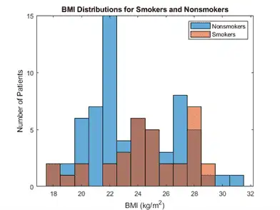
Create a histogram to explore whether there is a relationship between smoking and body-mass-index in this group of patients. You can index into BMI with the logical values from the Smoker table variable, because each row contains BMI and Smoker values for the same patient.

tf = (T.Smoker == false);
h1 = histogram(T.BMI(tf),'BinMethod','integers');
hold on
tf = (T.Smoker == true);
h2 = histogram(T.BMI(tf),'BinMethod','integers');
xlabel('BMI (kg/m^2)');
ylabel('Number of Patients');
legend('Nonsmokers','Smokers');
title('BMI Distributions for Smokers and Nonsmokers');
hold off

Add blood pressure readings for the patients from the workspace variables Systolic and Diastolic. Each row contains Systolic, Diastolic, and BMI values for the same patient.

T.Systolic = Systolic;
T.Diastolic = Diastolic;

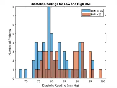
Create a histogram to show whether there is a relationship between high values of Diastolic and BMI.

tf = (T.BMI <= 25);
h1 = histogram(T.Diastolic(tf),'BinMethod','integers');
hold on
tf = (T.BMI > 25);
h2 = histogram(T.Diastolic(tf),'BinMethod','integers');
xlabel('Diastolic Reading (mm Hg)');
ylabel('Number of Patients');
legend('BMI <= 25','BMI > 25');
title('Diastolic Readings for Low and High BMI');
hold off

Reorder Table Variables and Rows for Output

To prepare the table for output, reorder the table rows by name, and table variables by position or name. Display the final arrangement of the table.

Sort the table by row names so that patients are listed in alphabetical order.

T = sortrows(T,'RowNames');

T(1:5,:)

ans=5×8 table
                   Gender      Smoker    Height    Weight     ID      BMI      Systolic    Diastolic
                 __________    ______    ______    ______    ____    ______    ________    _________

    Adams        {'Female'}    false       66       137      8235    22.112      127          83    
    Alexander    {'Male'  }    true        69       171      1300    25.252      128          99    
    Allen        {'Female'}    false       63       143      7432    25.331      113          80    
    Anderson     {'Female'}    false       68       128      1577    19.462      114          77    
    Bailey       {'Female'}    false       68       130      2239    19.766      113          81

Create a BloodPressure variable to hold blood pressure readings in a 100-by-2 table variable.

T.BloodPressure = [T.Systolic T.Diastolic];

Delete Systolic and Diastolic from the table since they are redundant.

T.Systolic = [];
T.Diastolic = [];

T(1:5,:)

ans=5×7 table
                   Gender      Smoker    Height    Weight     ID      BMI      BloodPressure
                 __________    ______    ______    ______    ____    ______    _____________

    Adams        {'Female'}    false       66       137      8235    22.112     127     83  
    Alexander    {'Male'  }    true        69       171      1300    25.252     128     99  
    Allen        {'Female'}    false       63       143      7432    25.331     113     80  
    Anderson     {'Female'}    false       68       128      1577    19.462     114     77  
    Bailey       {'Female'}    false       68       130      2239    19.766     113     81

To put ID as the first column, reorder the table variables by position.

T = T(:,[5 1:4 6 7]);

T(1:5,:)

ans=5×7 table
                  ID       Gender      Smoker    Height    Weight     BMI      BloodPressure
                 ____    __________    ______    ______    ______    ______    _____________

    Adams        8235    {'Female'}    false       66       137      22.112     127     83  
    Alexander    1300    {'Male'  }    true        69       171      25.252     128     99  
    Allen        7432    {'Female'}    false       63       143      25.331     113     80  
    Anderson     1577    {'Female'}    false       68       128      19.462     114     77  
    Bailey       2239    {'Female'}    false       68       130      19.766     113     81

You also can reorder table variables by name. To reorder the table variables so that Gender is last:

Find 'Gender' in the VariableNames property of the table.
Move 'Gender' to the end of a cell array of variable names.
Use the cell array of names to reorder the table variables.

varnames = T.Properties.VariableNames;
others = ~strcmp('Gender',varnames);
varnames = [varnames(others) 'Gender'];
T = T(:,varnames);

Display the first five rows of the reordered table.

T(1:5,:)

ans=5×7 table
                  ID     Smoker    Height    Weight     BMI      BloodPressure      Gender  
                 ____    ______    ______    ______    ______    _____________    __________

    Adams        8235    false       66       137      22.112     127     83      {'Female'}
    Alexander    1300    true        69       171      25.252     128     99      {'Male'  }
    Allen        7432    false       63       143      25.331     113     80      {'Female'}
    Anderson     1577    false       68       128      19.462     114     77      {'Female'}
    Bailey       2239    false       68       130      19.766     113     81      {'Female'}

Write Table to File

You can write the entire table to a file, or create a subtable to write a selected portion of the original table to a separate file.

Write T to a file with the writetable function.

writetable(T,'allPatientsBMI.txt');

You can use the readtable function to read the data in allPatientsBMI.txt into a new table.

Create a subtable and write the subtable to a separate file. Delete the rows that contain data on patients who are smokers. Then remove the Smoker variable. nonsmokers contains data only for the patients who are not smokers.

nonsmokers = T;
toDelete = (nonsmokers.Smoker == true);
nonsmokers(toDelete,:) = [];
nonsmokers.Smoker = [];

Write nonsmokers to a file.

writetable(nonsmokers,'nonsmokersBMI.txt');

Matlabsolutions.com provides guaranteed satisfaction with a commitment to complete the work within time. Combined with our meticulous work ethics and extensive domain experience, We are the ideal partner for all your homework/assignment needs. We pledge to provide 24*7 support to dissolve all your academic doubts. We are composed of 300+ esteemed Matlab and other experts who have been empanelled after extensive research and quality check.

Matlabsolutions.com provides undivided attention to each Matlab assignment order with a methodical approach to solution. Our network span is not restricted to US, UK and Australia rather extends to countries like Singapore, Canada and UAE. Our Matlab assignment help services include Image Processing Assignments, Electrical Engineering Assignments, Matlab homework help, Matlab Research Paper help, Matlab Simulink help. Get your work done at the best price in industry.