How Patch Data Relates to a Colormap

Relationship of the Colormap to x-, y-, and z-Coordinate Arrays

If you create a Patch object using x-, y-, and z-coordinate arrays, the CData property of the Patch object contains an indexing array C. This array controls the relationship between the colormap and your patch. To assign colors to the faces, specify C as an array with these characteristics:

Here is an example of C and its relationship to the colormap and three faces. The value of C(i) controls the color for the face defined by vertices (X(i,:), Y(i,:)).

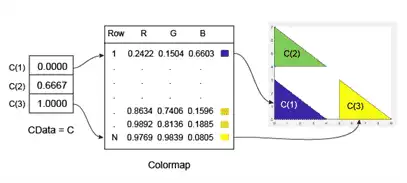
The smallest value in C is 0. It maps to the first row in the colormap. The largest value in C is 1, and it maps to the last row in the colormap. Intermediate values of C map linearly to the intermediate rows in the colormap. In this case, C(2) maps to the color located about two-thirds from the beginning of the colormap. This code creates the Patch object described in the preceding illustration.

X = [0 0 5; 0 0 5; 4 4 9];
Y = [0 4 0; 3 7 3; 0 4 0];
C = [0; .6667; 1];
p = patch(X,Y,C);
colorbar

To assign colors to the vertices, specify C as an array with these characteristics:

Here is an example of C and its relationship to the colormap and six vertices. The value of C(i,j) controls the color for the vertex at (X(i,j), Y(i,j)).

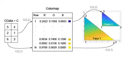
As with patch faces, MATLAB^® scales the values in C to the number of rows in the colormap. In this case, the smallest value is C(2,2)=1, and it maps to the first row in the colormap. The largest value is C(3,1)=6, and it maps to the last row in the colormap.

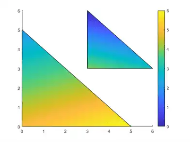
This code creates the Patch object described in the preceding illustration. The FaceColor property is set to 'interp' to make the vertex colors blend across each face.

clf
X = [0 3; 0 3; 5 6];
Y = [0 3; 5 6; 0 3];
C = [5 4; 2 0; 6 3];
p = patch(X,Y,C,'FaceColor','interp');
colorbar

Relationship of the Colormap to Face-Vertex Data

If you create patches using face-vertex data, the FaceVertexCData property of the Patch object contains an indexing array C. This array controls the relationship between the colormap and your patch.

To assign colors to the faces, specify C as an array with these characteristics:

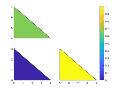
Here is an example of C and its relationship to the colormap and three faces.

The smallest value in C is 0, and it maps to the first row in the colormap. The largest value in C is 1, and it maps to the last value in the colormap. Intermediate values of C map linearly to the intermediate rows in the colormap. In this case, C(2) maps to the color located about two-thirds from the bottom of the colormap.

This code creates the Patch object described in the preceding illustration. The FaceColor property is set to 'flat' to display the colormap colors instead of the default color, which is black.

clf
vertices = [0 0; 0 3; 4 0; 0 4; 0 7; 4 4; 5 0; 5 3; 9 0];
faces = [1 2 3; 4 5 6; 7 8 9];
C = [0; 0.6667; 1];
p = patch('Faces',faces,'Vertices',vertices,'FaceVertexCData',C);
p.FaceColor = 'flat';
colorbar

To assign colors to the vertices, specify the FaceVertexCData property of the Patch object as array C with these characteristics:

Here is an example of C and its relationship to the colormap and six vertices.

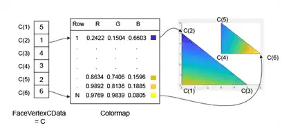
As with patch faces, MATLAB scales the values in C to the number of rows in the colormap. In this case, the smallest value is C(2)=1, and it maps to the first row in the colormap. The largest value is C(6)=6, and it maps to the last row in the colormap.

This code creates the Patch object described in the preceding illustration. The FaceColor property is set to 'interp' to make the vertex colors blend across each face.

clf
vertices = [0 0; 0 5; 5 0; 3 3; 3 6; 6 3];
faces = [1 2 3; 4 5 6];
C = [5; 1; 4; 3; 2; 6];
p = patch('Faces',faces,'Vertices',vertices,'FaceVertexCData',C);
p.FaceColor = 'interp';
colorbar