This example shows how to visualize and measure signals in the time and frequency domain in MATLAB® using a time scope and spectrum analyzer.
Signal Visualization in Time and Frequency Domains
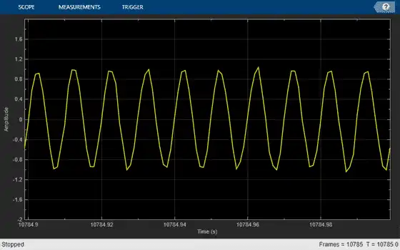
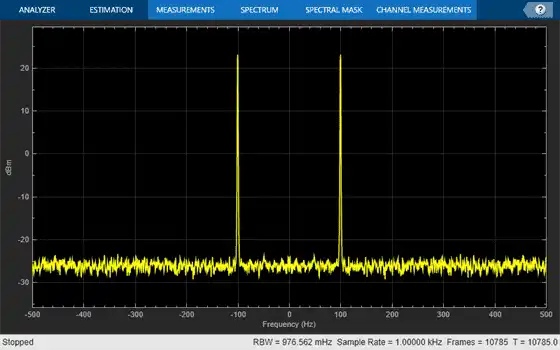
Create a sine wave with a frequency of 100 Hz sampled at 1000 Hz. Generate five seconds of the 100 Hz sine wave with additive N(0,0.0025) white noise in one-second intervals. Send the signal to a time scope and spectrum analyzer for display and measurement.
SampPerFrame = 1000;
Fs = 1000;
SW = dsp.SineWave('Frequency',100,...
  'SampleRate',Fs,...
  'SamplesPerFrame',SampPerFrame);
TS = timescope('SampleRate',Fs,...
    'TimeSpanSource','property',...
    'TimeSpan',0.1,...
    'YLimits',[-2, 2],...
    'ShowGrid',true);
SA = spectrumAnalyzer('SampleRate',Fs,...
    'Method','welch','AveragingMethod','exponential');
tic;
while toc < 10
  sigData = SW() + 0.05*randn(SampPerFrame,1);
  SA(sigData);
  TS(sigData);
end
release(TS)
release(SA)
Time-Domain Measurements
Using the time scope, you can make a number of time-domain signal measurements.
The following measurements are available:
-
Cursor Measurements - Puts screen cursors on all scope displays.
-
Signal Statistics - Displays maximum, minimum, peak-to-peak difference, mean, median, RMS values of a selected signal, and the times at which the maximum and minimum occur.
-
Bilevel Measurements - Displays information about a selected signal's transitions, aberrations, and cycles.
-
Peak Finder - Displays maxima and the times at which they occur.
You can enable and disable these measurements from the Measurements tab.
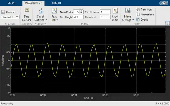
To illustrate the use of measurements in the time scope, simulate an ECG signal. Use the ecg function to generate 2700 samples of the signal. Use a Savitzky-Golay filter to smooth the signal and periodically extend the data to obtain approximately 11 periods.
x = 3.5*ecg(2700).';
y = repmat(sgolayfilt(x,0,21),[1 13]);
sigData = y((1:30000) + round(2700*rand(1))).';
Display the signal in the time scope and use the Peak Finder and Data Cursor measurements. Assume a sample rate of 4 kHz.
TS_ECG = timescope('SampleRate',4000,...
    'TimeSpanSource','Auto',...
    'ShowGrid', true);
TS_ECG(sigData);
TS_ECG.YLimits = [-4, 4];
Peak Measurements
Enable Peak Measurements from the Measurements tab by clicking the corresponding toolstrip button. The Peaks pane appears at the bottom of the time scope window. For the Num Peaks property, enter 8 and press Enter. In the Peaks pane, the time scope displays a list of 8 peak amplitude values and the times at which they occur.
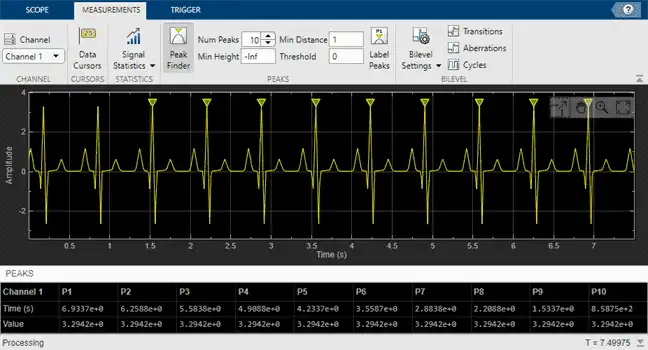
There is a constant time difference of 0.675 seconds between each heartbeat. Therefore, the heart rate of the ECG signal is given by the following equation:
60sec/min0.675sec/beat=88.89beats/min(bpm)
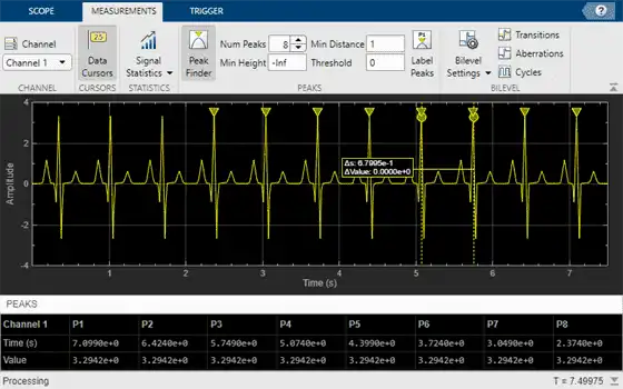
Cursor Measurements
Enable Cursor Measurements from the Measurements tab by clicking the corresponding toolstrip button. The cursors appear on the time scope with a box showing the change in time and value between the two cursors. You can drag the cursors and use them to measure the time between events in the waveform. As you drag a cursor, the time an value at the cursor appears. This figure shows how to use cursors to measure the time interval between peaks in the ECG waveform. The ΔT measurement in the cursor box demonstrates that the time interval between the two peaks is 0.675 seconds corresponding to a heart rate of 1.482 Hz or 88.9 beats/min.
Signal Statistics and Bilevel Measurements
You can also select Signal Statistics and various bilevel measurements from the Measurements tab. Signal Statistics can be used to determine the signal's minimum and maximum values as well as other metrics like the peak-to-peak, mean, median, and RMS values. Bilevel measurements can be used to determine information about rising and falling transitions, transition aberrations, overshoot and undershoot information, settling time, pulse width, and duty cycle. To read more about these measurements, see Configure Time Scope MATLAB Object.
Frequency-Domain Measurements
This section explains how to make frequency domain measurements with the spectrum analyzer.
The spectrum analyzer provides the following measurements:
-
Cursor Measurements - places cursors on the spectrum display.
-
Peak Finder - displays maxima and the frequencies at which they occur.
-
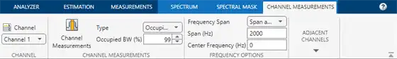
Channel Measurements - displays occupied bandwidth and ACPR channel measurements.
-
Distortion Measurements - displays harmonic and intermodulation distortion measurements.
You can enable and disable these measurements from the spectrum analyzer toolstrip.
Distortion Measurements
To illustrate the use of measurements with the spectrum analyzer, create a 2.5 kHz sine wave sampled at 48 kHz with additive white Gaussian noise. Evaluate a high-order polynomial (9th degree) at each signal value to model non-linear distortion. Display the signal in a spectrum analyzer.
Fs = 48e3;
SW = dsp.SineWave('Frequency',2500,...
  'SampleRate',Fs,...
  'SamplesPerFrame',SampPerFrame);

SA_Distortion = spectrumAnalyzer('SampleRate',Fs,...
    'Method','welch',...
    'AveragingMethod','exponential',...
    'PlotAsTwoSidedSpectrum',false);
y = [1e-6 1e-9 1e-5 1e-9 1e-6 5e-8 0.5e-3 1e-6 1 3e-3];
tic;
while toc < 5
  x = SW() + 1e-8*randn(SampPerFrame,1);
  sigData = polyval(y, x);
  SA_Distortion(sigData);
end
release(SA_Distortion);
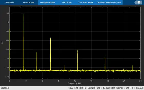
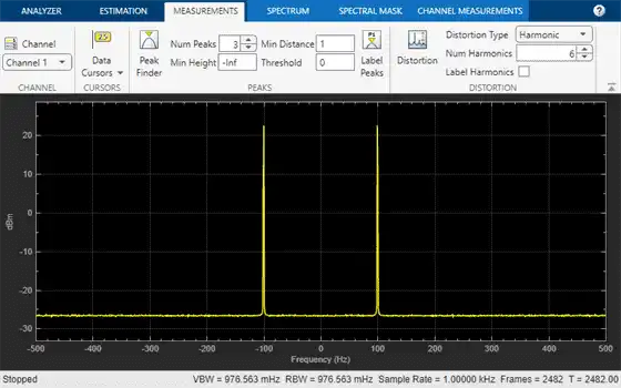
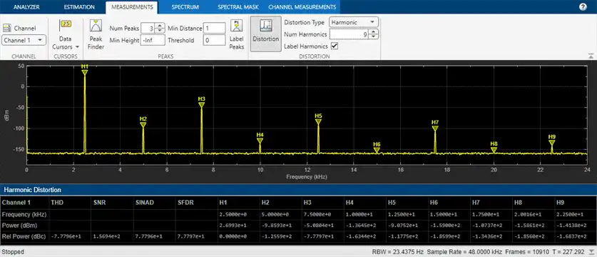
Enable the harmonic distortion measurements by selecting the Distortion button on the Measurements tab of the spectrum analyzer toolstrip. In the Distortion section, change the value for Num Harmonics to 9 and check the Label Harmonics checkbox. In the Harmonic Distortion panel at the bottom of the spectrum analyzer window, you see the value of the fundamental close to 2500 Hz and 8 harmonics as well as their SNR, SINAD, THD and SFDR values, which are referenced with respect to the fundamental output power.
Peak Finder
You can track time-varying spectral components by using the Peak Finder measurements. You can show and optionally label up to 100 peaks. To invoke the Peak Finder, select the Peak Finder button on the Measurements tab of the spectrum analyzer toolstrip.
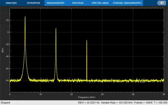
To illustrate the use of Peak Finder, create a signal consisting of the sum of three sine waves with frequencies of 5, 15, and 25 kHz and amplitudes of 1, 0.1, and 0.01 respectively. The data is sampled at 100 kHz. Add N(0,10−8) white Gaussian noise to the sum of sine waves and display the one-sided power spectrum in the spectrum analyzer.
Fs = 100e3;
SW1 = dsp.SineWave(1e0,5e3,0,...
    'SampleRate',Fs,...
    'SamplesPerFrame',SampPerFrame);
SW2 = dsp.SineWave(1e-1,15e3,0,...
    'SampleRate',Fs,...
    'SamplesPerFrame',SampPerFrame);
SW3 = dsp.SineWave(1e-2,25e3,0,...
    'SampleRate',Fs,...
    'SamplesPerFrame',SampPerFrame);

SA_Peak = spectrumAnalyzer('SampleRate',Fs,...
    'Method','welch',...
    'AveragingMethod','exponential',...
    'PlotAsTwoSidedSpectrum',false);
tic;
while toc < 10
    sigData = SW1() + SW2() + SW3() + 1e-4*randn(SampPerFrame,1);
    SA_Peak(sigData);
end
release(SA_Peak);
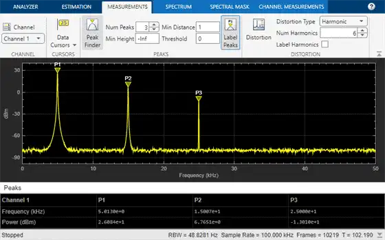
Enable the Peak Finder to label the three sine wave frequencies. The frequency values and powers in dBm are displayed below the plot. You can increase or decrease the maximum number of peaks, specify a minimum peak distance, and change other settings in the Peaks section of the Measurements tab.
To learn more about the use of measurements with the spectrum analyzer, see the Spectrum Analyzer Measurements example.