App Workflow
A typical workflow for inspecting and comparing signals using the Signal Analyzer app is:
-
Select Signals to Analyze — Select any signal available in the MATLAB® workspace. The app accepts numeric arrays and signals with inherent time information, such as MATLAB
timetablearrays,timeseriesobjects, andlabeledSignalSetobjects. See Data Types Supported by Signal Analyzer for more information. -
Preprocess Signals — Lowpass, highpass, bandpass, or bandstop filter signals. Remove trends and compute signal envelopes. Smooth signals using moving averages, regression, Savitzky-Golay filters, or other methods. Change sample rates of signals or interpolate nonuniformly sampled signals onto uniform grids. Preprocess signals using your own custom functions. Generate MATLAB functions to automate preprocessing operations.
-
Explore Signals — Add time information to signals using sample rates, numeric vectors,
durationarrays, or MATLAB expressions. Plot, measure, and compare data, their spectra, their spectrograms, or their scalograms. Look for features and patterns in the time domain, in the frequency domain, and in the time-frequency domain. Compute persistence spectra to analyze sporadic signals and sharpen spectrogram estimates using reassignment. Extract regions of interest from signals. -
Share Analysis — Copy displays from the app to the clipboard as images. Export signals to the MATLAB workspace or save them to MAT-files. Generate MATLAB scripts to automate the computation of power spectrum, spectrogram, or persistence spectrum estimates and the extraction of regions of interest. Save Signal Analyzer sessions to resume your analysis later or on another machine.
Example: Extract Regions of Interest from Whale Song
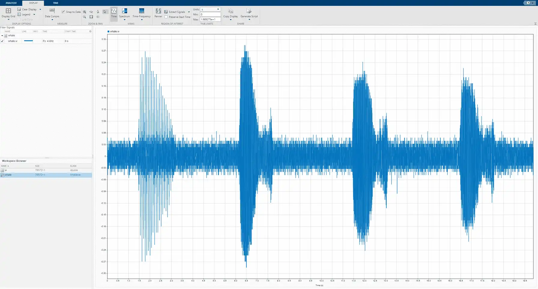
Load a file that contains audio data from a Pacific blue whale, sampled at 4 kHz. The file is from the library of animal vocalizations maintained by the Cornell University Bioacoustics Research Program. The time scale in the data is compressed by a factor of 10 to raise the pitch and make the calls more audible. Convert the signal to a MATLAB® timetable.
whaleFile = fullfile(matlabroot,'examples','matlab','data','bluewhale.au');
[w,fs] = audioread(whaleFile);

whale = timetable(seconds((0:length(w)-1)'/fs),w);

% To hear, type soundsc(w,fs)
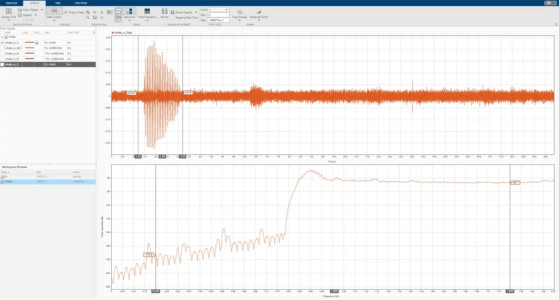
Open Signal Analyzer and drag the timetable to a display. Four features stand out from the noise. The first is known as a trill, and the other three are known as moans.
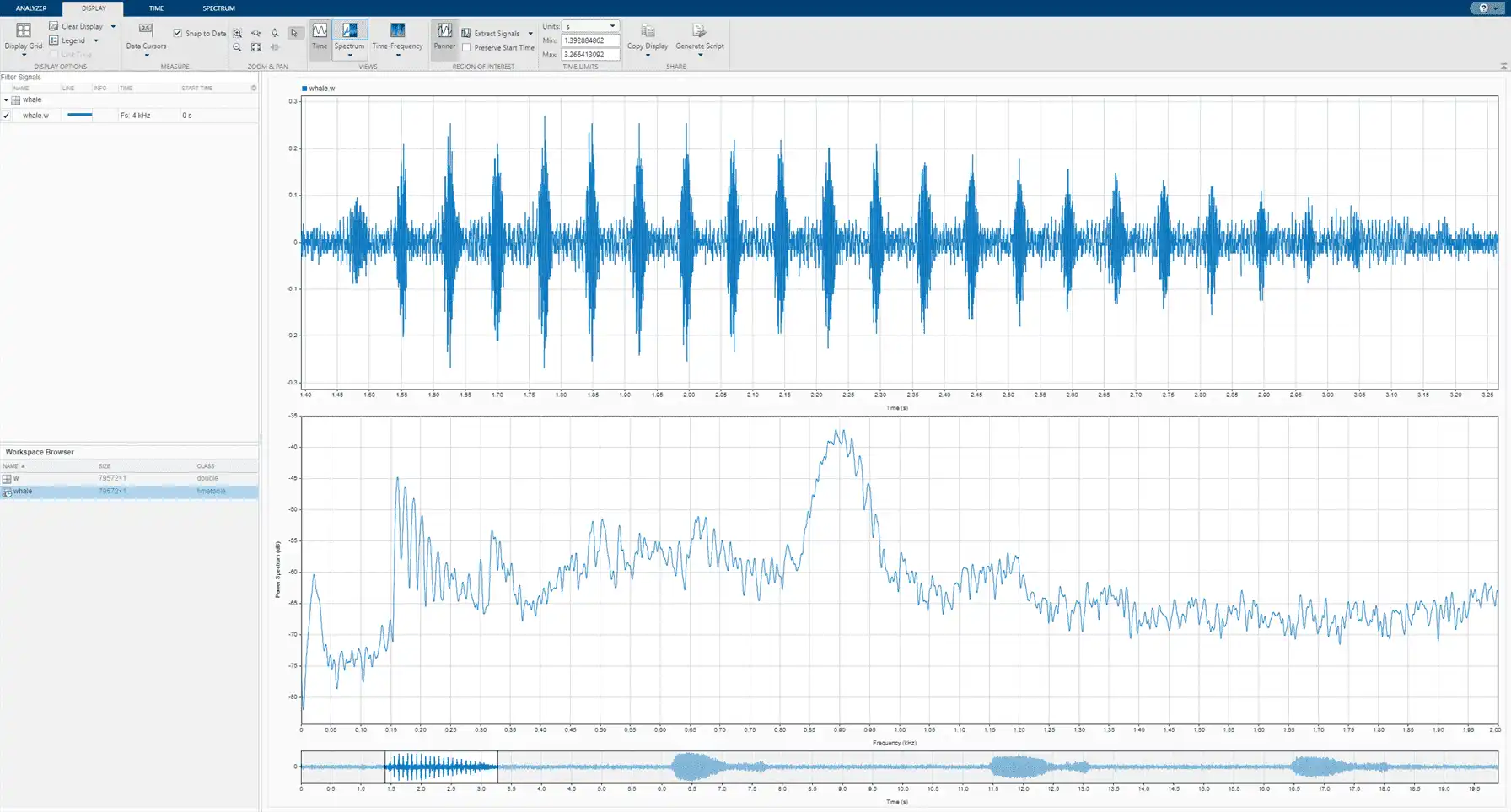
On the Display tab, click Spectrum to open a spectrum view and click Panner to activate the panner. Use the panner to create a zoom window with a width of about 2 seconds. Drag the zoom window so that it is centered on the trill. The spectrum shows a noticeable peak at around 900 Hz.
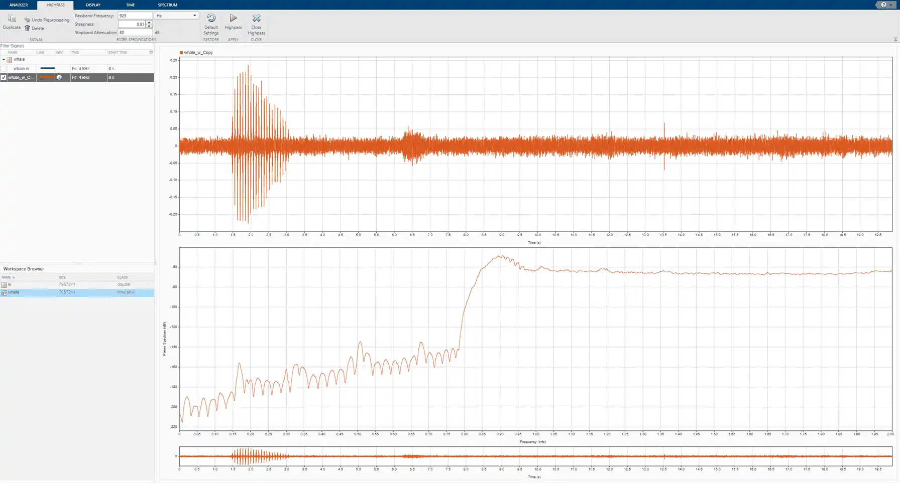
Isolate the single trill by highpass filtering. Right-click the signal in the Signal table and select Duplicate to create a copy of the whale song. Remove the original signal from the display by clearing the check box next to its name in the Signal table. On the Analyzer tab, click Preprocessing ? and select Highpass. Set the passband frequency to 925 Hz and the stopband attenuation at 80 dB. Use the default value for the steepness.
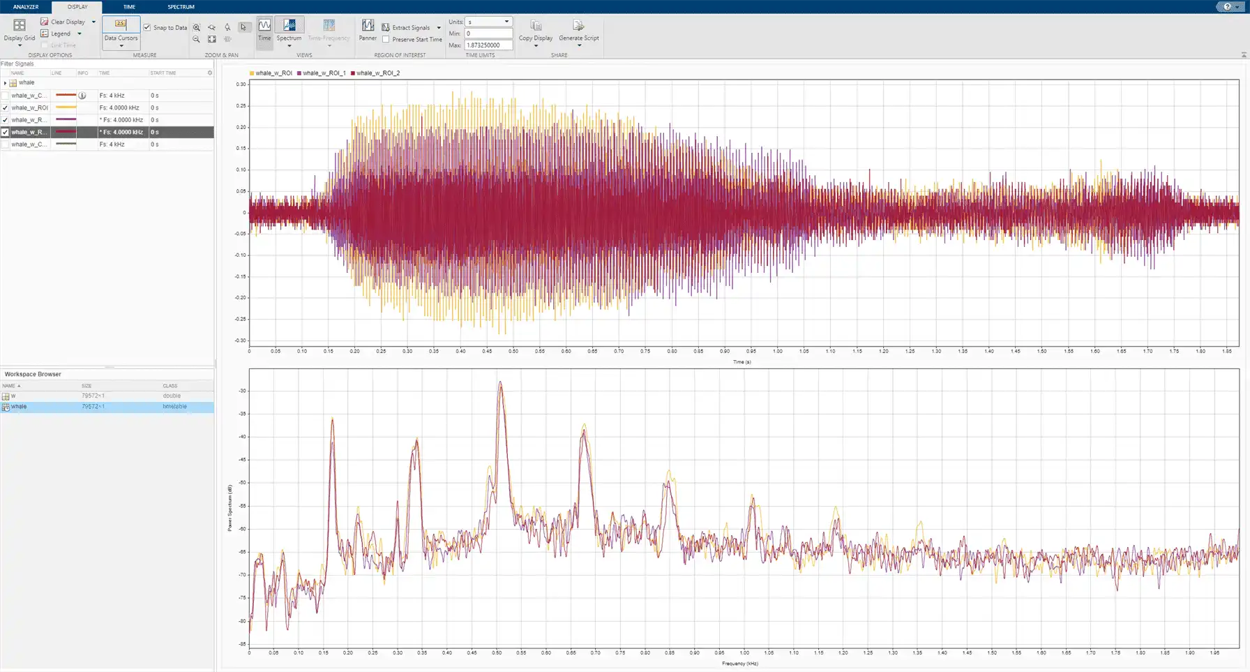
Clear the display and select the original signal. Extract the three moans to compare their spectra:
-
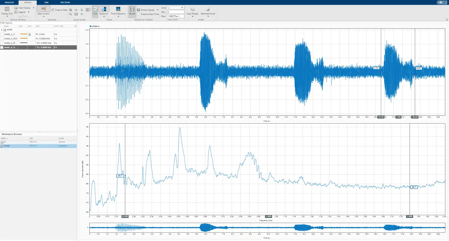
Center the panner zoom window on the first moan. The spectrum has eight clearly defined peaks, located very close to multiples of 170 Hz. Click Extract Signals ? and select
Between Time Limits. -
Click Panner to hide the panner. Press the space bar to see the full signal. Click Zoom in X and zoom in on a 2-second interval of the time view centered on the second moan. The spectrum again has peaks at multiples of 170 Hz. Click Extract Signals ? and select
Between Time Limits. -
Press the space bar to see the full signal. Click Data Cursors ? and select
Two. Place the time domain cursors in a 2-second interval around the third moan. Again, there are peaks at multiples of 170 Hz. Click Extract Signals ? and selectBetween Time Cursors.
Plot the highpass-filtered signal and place the two data cursors at 1 second and 3.5 seconds. Extract the region containing the trill.
Remove the original signal from the display by clearing the check box next to its name in the Signal table. Display the three regions of interest you just extracted. Their spectra lie approximately on top of each other.
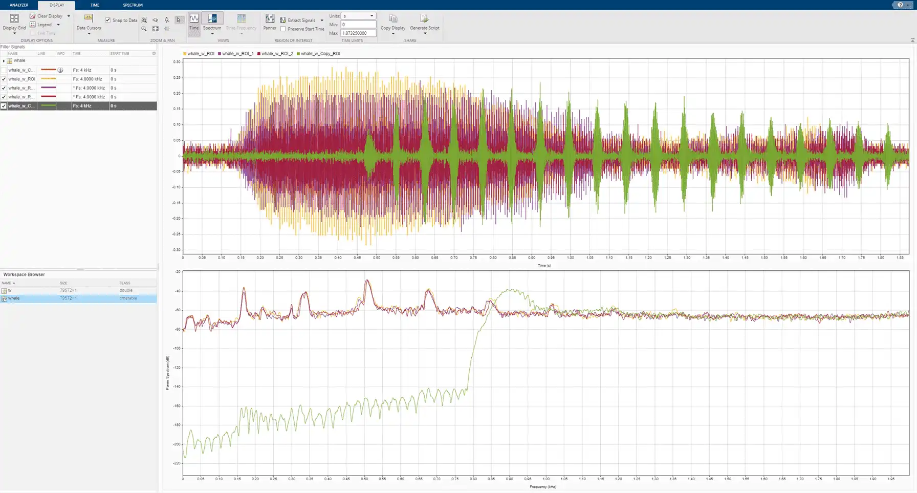
On the same display, plot the region of interest containing the trill that you extracted. The trill and moan spectra are noticeably different.
Click on Export on the Analyzer tab to export the four regions of interest in a MAT-file.