View the Spectrogram Using Spectrum Analyzer

Spectrograms are a two-dimensional representation of the power spectrum of a signal as this signal sweeps through time. They give a visual understanding of the frequency content of your signal. Each line of the spectrogram is one periodogram computed using either the filter bank approach or the Welch’s algorithm of averaging modified periodogram.

To show the concepts of the spectrogram, this example uses the model ex_psd_sa as the starting point.

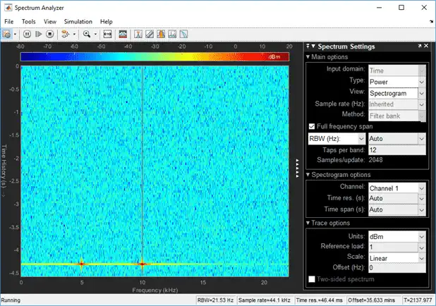
Open the model and double-click the Spectrum Analyzer block. In the Spectrum Settings pane, change View to Spectrogram. The Method is set to Filter bank. Run the model. You can see the spectrogram output in the spectrum analyzer window. To acquire and store the data for further processing, create a SpectrumAnalyzerConfiguration object and run the getSpectrumData function on this object.

Colormap

Power spectrum is computed as a function of frequency f and is plotted as a horizontal line. Each point on this line is given a specific color based on the value of the power at that particular frequency. The color is chosen based on the colormap seen at the top of the display. To change the colormap, click View > Configuration Properties, and choose one of the options in color map. Make sure View is set to Spectrogram. By default, color map is set to jet(256).

The two frequencies of the sine wave are distinctly visible at 5 kHz and 10 kHz. Since the spectrum analyzer uses the filter bank approach, there is no spectral leakage at the peaks. The sine wave is embedded in Gaussian noise, which has a variance of 0.0001. This value corresponds to a power of -40 dBm. The color that maps to -40 dBm is assigned to the noise spectrum. The power of the sine wave is 26.9 dBm at 5 kHz and 10 kHz. The color used in the display at these two frequencies corresponds to 26.9 dBm on the colormap. For more information on how the power is computed in dBm, see 'Conversion of power in watts to dBW and dBm'.

To confirm the dBm values, change View to Spectrum. This view shows the power of the signal at various frequencies.

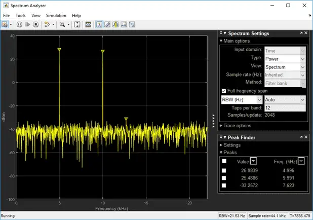
You can see that the two peaks in the power display have an amplitude of about 26 dBm and the white noise is averaging around -40 dBm.

Display

In the spectrogram display, time scrolls from top to bottom, so the most recent data is shown at the top of the display. As the simulation time increases, the offset time also increases to keep the vertical axis limits constant while accounting for the incoming data. The Offset value, along with the simulation time, is displayed at the bottom-right corner of the spectrogram scope.

Resolution Bandwidth (RBW)

Resolution Bandwidth (RBW) is the minimum frequency bandwidth that can be resolved by the spectrum analyzer. By default, RBW (Hz) is set to Auto. In the auto mode, RBW is the ratio of the frequency span to 1024. In a two-sided spectrum, this value is F_s/1024, while in a one-sided spectrum, it is (F_s/2)/1024. In this example, RBW is (44100/2)/1024 or 21.53 Hz.

If the Method is set to Filter bank, using this value of RBW, the number of input samples used to compute one spectral update is given by N_samples = F_s/RBW, which is 44100/21.53 or 2048 in this example.

If the Method is set to Welch, using this value of RBW, the window length (N_samples) is computed iteratively using this relationship:

O_p is the amount of overlap between the previous and current buffered data segments. NENBW is the equivalent noise bandwidth of the window.

For more information on the details of the spectral estimation algorithm, see Spectral Analysis.

To distinguish between two frequencies in the display, the distance between the two frequencies must be at least RBW. In this example, the distance between the two peaks is 5000 Hz, which is greater than RBW. Hence, you can see the peaks distinctly.

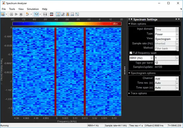
Change the frequency of the second sine wave from 10000 Hz to 5015 Hz. The difference between the two frequencies is 15 Hz, which is less than RBW.

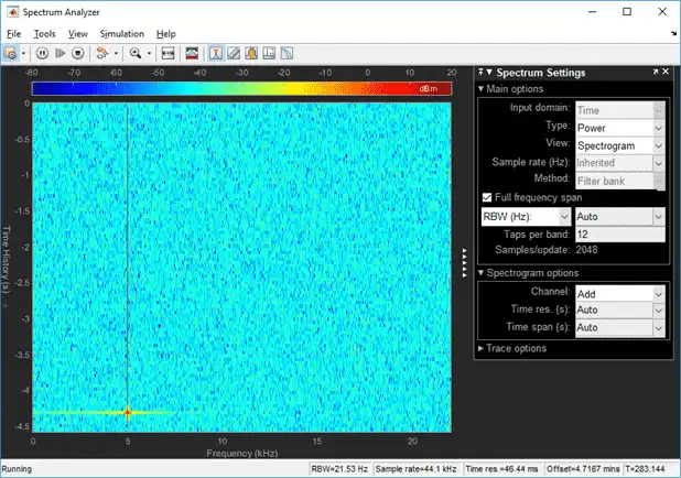
On zooming, you can see that the peaks at 5000 Hz and 5015 Hz are not distinguishable.

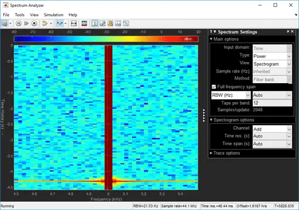
To increase the frequency resolution, decrease RBW to 1 Hz and run the simulation. On zooming, the two peaks, which are 15 Hz apart, are now distinguishable

Time Resolution

Time resolution is the distance between two spectral lines in the vertical axis. By default, Time res (s) is set to Auto. In this mode, the value of time resolution is 1/RBW s, which is the minimum attainable resolution. When you increase the frequency resolution, the time resolution decreases. To maintain a good balance between the frequency resolution and time resolution, change the RBW (Hz) to Auto. You can also specify the Time res (s) as a numeric value.

Convert the Power Between Units

The spectrum analyzer provides three units to specify the power spectral density: Watts/Hz, dBm/Hz, and dBW/Hz. Corresponding units of power are Watts, dBm, and dBW. For electrical engineering applications, you can also view the RMS of your signal in Vrms or dBV. The default spectrum type is Power in dBm.

Convert the Power in Watts to dBW and dBm

Power in dBW is given by:

Power in dBm is given by:

For a sine wave signal with an amplitude of 1 V, the power of a one-sided spectrum in Watts is given by:

In this example, this power equals 0.5 W. Corresponding power in dBm is given by:

Here, the power equals 26.9897 dBm. To confirm this value with a peak finder, click Tools > Measurements > Peak Finder.

For a white noise signal, the spectrum is flat for all frequencies. The spectrum analyzer in this example shows a one-sided spectrum in the range [0 Fs/2]. For a white noise signal with a variance of 1e-4, the power per unit bandwidth (P_{unitbandwidth}) is 1e-4. The total power of white noise in watts over the entire frequency range is given by:

The number of frequency bins is the ratio of total bandwidth to RBW. For a one-sided spectrum, the total bandwidth is half the sampling rate. RBW in this example is 21.53 Hz. With these values, the total power of white noise in watts is 0.1024 W. In dBm, the power of white noise can be calculated using 10*log10(0.1024/10^-3), which equals 20.103 dBm.

Convert Power in Watts to dBFS

If you set the spectral units to dBFS and set the full scale (FullScaleSource) to Auto, power in dBFS is computed as:

where:

If you specify a manual full scale (set FullScaleSource to Property), power in dBFS is given by:

Where FS is the full scaling factor specified in the FullScale property.

For a sine wave signal with an amplitude of 1 V, the power of a one-sided spectrum in Watts is given by:

In this example, this power equals 0.5 W and the maximum input signal for a sine wave is 1 V. The corresponding power in dBFS is given by:

Here, the power equals -3.0103. To confirm this value in the spectrum analyzer, run these commands:

Fs = 1000;  % Sampling frequency
sinef = dsp.SineWave('SampleRate',Fs,'SamplesPerFrame',100);
scope = dsp.SpectrumAnalyzer('SampleRate',Fs,...
   'SpectrumUnits','dBFS','PlotAsTwoSidedSpectrum',false)
%%
for ii = 1:100000
xsine = sinef();
scope(xsine)
end

Then, click Tools > Measurements > Peak Finder.

Convert the Power in dBm to RMS in Vrms

Power in dBm is given by:

Voltage in RMS is given by:

From the previous example, P_dBm equals 26.9897 dBm. The V_rms is calculated as

which equals 0.7071.

To confirm this value:

Scale Color Limits

When you run the model and do not see the spectrogram colors, click the Scale Color Limits  button. This option autoscales the colors.

The spectrogram updates in real time. During simulation, if you change any of the tunable parameters in the model, the changes are effective immediately in the spectrogram.