Waveform Segmentation Using Deep Learning

Introduction

The electrical activity in the human heart can be measured as a sequence of amplitudes away from a baseline signal. For a single normal heartbeat cycle, the ECG signal can be divided into the following beat morphologies [1]:

The segmentation of these regions of ECG waveforms can provide the basis for measurements useful for assessing the overall health of the human heart and the presence of abnormalities [2]. Manually annotating each region of the ECG signal can be a tedious and time-consuming task. Signal processing and deep learning methods potentially can help streamline and automate region-of-interest annotation.

This example uses ECG signals from the publicly available QT Database [3] [4]. The data consists of roughly 15 minutes of ECG recordings, with a sample rate of 250 Hz, measured from a total of 105 patients. To obtain each recording, the examiners placed two electrodes on different locations on a patient's chest, resulting in a two-channel signal. The database provides signal region labels generated by an automated expert system [2]. This example aims to use a deep learning solution to provide a label for every ECG signal sample according to the region where the sample is located. This process of labeling regions of interest across a signal is often referred to as waveform segmentation.

To train a deep neural network to classify signal regions, you can use a Long Short-Term Memory (LSTM) network. This example shows how signal preprocessing techniques and time-frequency analysis can be used to improve LSTM segmentation performance. In particular, the example uses the Fourier synchrosqueezed transform to represent the nonstationary behavior of the ECG signal.

Download and Prepare the Data

Each channel of the 105 two-channel ECG signals was labeled independently by the automated expert system and is treated independently, for a total of 210 ECG signals that were stored together with the region labels in 210 MAT-files. The files are available at the following location: https://www.mathworks.com/supportfiles/SPT/data/QTDatabaseECGData.zip.

Download the data files into your temporary directory, whose location is specified by MATLAB®'s tempdir command. If you want to place the data files in a folder different from tempdir, change the directory name in the subsequent instructions.

% Download the data
dataURL = 'https://www.mathworks.com/supportfiles/SPT/data/QTDatabaseECGData1.zip';
datasetFolder = fullfile(tempdir,'QTDataset');
zipFile = fullfile(tempdir,'QTDatabaseECGData.zip');
if ~exist(datasetFolder,'dir')
     websave(zipFile,dataURL);
     unzip(zipFile,tempdir);
end

The unzip operation creates the QTDatabaseECGData folder in your temporary directory with 210 MAT-files in it. Each file contains an ECG signal in variable ecgSignal and a table of region labels in variable signalRegionLabels. Each file also contains the sample rate of the signal in variable Fs. In this example all signals have a sample rate of 250 Hz.

Create a signal datastore to access the data in the files. This example assumes the dataset has been stored in your temporary directory under the QTDatabaseECGData folder. If this is not the case, change the path to the data in the code below. Specify the signal variable names you want to read from each file using the SignalVariableNames parameter.

sds = signalDatastore(datasetFolder,'SignalVariableNames',["ecgSignal","signalRegionLabels"])

sds = 
  signalDatastore with properties:

                       Files:{
                             '/tmp/QTDataset/ecg1.mat';
                             '/tmp/QTDataset/ecg10.mat';
                             '/tmp/QTDataset/ecg100.mat'
                              ... and 207 more
                             }
    AlternateFileSystemRoots: [0×0 string]
                    ReadSize: 1
         SignalVariableNames: ["ecgSignal"    "signalRegionLabels"]

The datastore returns a two-element cell array with an ECG signal and a table of region labels each time you call the read function. Use the preview function of the datastore to see that the content of the first file is a 225,000 samples long ECG signal and a table containing 3385 region labels.

data = preview(sds)

data=2×1 cell array
    {225000×1 double}
    {  3385×2 table }

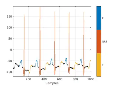
Look at the first few rows of the region labels table and observe that each row contains the region limit indices and the region class value (P, T, or QRS).

head(data{2})

ans=8×2 table
    ROILimits     Value
    __________    _____

     83    117     P   
    130    153     QRS 
    201    246     T   
    285    319     P   
    332    357     QRS 
    412    457     T   
    477    507     P   
    524    547     QRS 

Visualize the labels for the first 1000 samples using a signalMask object.

M = signalMask(data{2});
plotsigroi(M,data{1}(1:1000))

The usual machine learning classification procedure is the following:

The network is trained with 70% of the data and tested with the remaining 30%.

For reproducible results, reset the random number generator. Use the dividerand function to get random indices to shuffle the files, and the subset function of signalDatastore to divide the data into training and testing datastores.

rng default
[trainIdx,~,testIdx] = dividerand(numel(sds.Files),0.7,0,0.3);
trainDs = subset(sds,trainIdx);
testDs = subset(sds,testIdx);

In this segmentation problem, the input to the LSTM network is an ECG signal and the output is a sequence or mask of labels with the same length as the input signal. The network task is to label each signal sample with the name of the region it belongs to. For this reason, it is necessary to transform the region labels on the dataset to sequences containing one label per signal sample. Use a transformed datastore and the getmask helper function to transform the region labels. The getmask function adds a label category, "n/a", to label samples that do not belong to any region of interest.

type getmask.m

function outputCell = getmask(inputCell)
%GETMASK Convert region labels to a mask of labels of size equal to the
%size of the input ECG signal.
%
%   inputCell is a two-element cell array containing an ECG signal vector
%   and a table of region labels. 
%
%   outputCell is a two-element cell array containing the ECG signal vector
%   and a categorical label vector mask of the same length as the signal. 

% Copyright 2020 The MathWorks, Inc.

sig = inputCell{1};
roiTable = inputCell{2};
L = length(sig);
M = signalMask(roiTable);

% Get categorical mask and give priority to QRS regions when there is overlap
mask = catmask(M,L,'OverlapAction','prioritizeByList','PriorityList',[2 1 3]);

% Set missing values to "n/a"
mask(ismissing(mask)) = "n/a";

outputCell = {sig,mask};
end

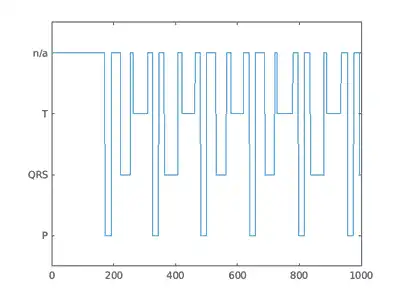
Preview the transformed datastore to observe that it returns a signal vector and a label vector of equal lengths. Plot the first 1000 element of the categorical mask vector.

trainDs = transform(trainDs, @getmask);
testDs = transform(testDs, @getmask);

transformedData = preview(trainDs)

transformedData=1×2 cell array
    {224993×1 double}    {224993×1 categorical}

plot(transformedData{2}(1:1000))

Passing very long input signals into the LSTM network can result in estimation performance degradation and excessive memory usage. To avoid these effects, break the ECG signals and their corresponding label masks using a transformed datastore and the resizeData helper function. The helper function creates as many 5000-sample segments as possible and discards the remaining samples. A preview of the output of the transformed datastore shows that the first ECG signal and its label mask are broken into 5000-sample segments. Note that preview of the transformed datastore only shows the first 8 elements of the otherwise floor(224993/5000) = 44 element cell array that would result if we called the datastore read function.

trainDs = transform(trainDs,@resizeData);
testDs = transform(testDs,@resizeData);
preview(trainDs)

ans=8×2 cell array
    {1×5000 double}    {1×5000 categorical}
    {1×5000 double}    {1×5000 categorical}
    {1×5000 double}    {1×5000 categorical}
    {1×5000 double}    {1×5000 categorical}
    {1×5000 double}    {1×5000 categorical}
    {1×5000 double}    {1×5000 categorical}
    {1×5000 double}    {1×5000 categorical}
    {1×5000 double}    {1×5000 categorical}

Choose to Train Networks or Download Pre-Trained Networks

The next sections of this example compare three different approaches to train LSTM networks. Due to the large size of the dataset, the training process of each network may take several minutes. If your machine has a GPU and Parallel Computing Toolbox™, then MATLAB automatically uses the GPU for faster training. Otherwise, it uses the CPU.

You can skip the training steps and download the pre-trained networks using the selector below. If you want to train the networks as the example runs, select 'Train Networks'. If you want to skip the training steps, select 'Download Networks' and a file containing all three pre-trained networks -rawNet, filteredNet, and fsstNet- will be downloaded into your temporary directory, whose location is specified by MATLAB®'s tempdir command. If you want to place the downloaded file in a folder different from tempdir, change the directory name in the subsequent instructions.

actionFlag = "Train networks";
if actionFlag == "Download networks"
    % Download the pre-trained networks
    dataURL = 'https://ssd.mathworks.com/supportfiles/SPT/data/QTDatabaseECGSegmentationNetworks.zip'; %#ok<*UNRCH>
    modelsFolder = fullfile(tempdir,'QTDatabaseECGSegmentationNetworks');
    modelsFile = fullfile(modelsFolder,'trainedNetworks.mat');
    zipFile = fullfile(tempdir,'QTDatabaseECGSegmentationNetworks.zip');
    if ~exist(modelsFolder,'dir')
        websave(zipFile,dataURL);
        unzip(zipFile,fullfile(tempdir,'QTDatabaseECGSegmentationNetworks'));
    end
    load(modelsFile)
end

Results between the downloaded networks and newly trained networks may vary slightly since the networks are trained using random initial weights.

Input Raw ECG Signals Directly into the LSTM Network

First, train an LSTM network using the raw ECG signals from the training dataset.

Define the network architecture before training. Specify a sequenceInputLayer of size 1 to accept one-dimensional time series. Specify an LSTM layer with the 'sequence' output mode to provide classification for each sample in the signal. Use 200 hidden nodes for optimal performance. Specify a fullyConnectedLayer with an output size of 4, one for each of the waveform classes. Add a softmaxLayer and a classificationLayer to output the estimated labels.

layers = [ ...
    sequenceInputLayer(1)
    lstmLayer(200,'OutputMode','sequence')
    fullyConnectedLayer(4)
    softmaxLayer
    classificationLayer];

Choose options for the training process that ensure good network performance. Refer to the trainingOptions (Deep Learning Toolbox) documentation for a description of each parameter.

options = trainingOptions('adam', ...
    'MaxEpochs',10, ...
    'MiniBatchSize',50, ...
    'InitialLearnRate',0.01, ...
    'LearnRateDropPeriod',3, ...
    'LearnRateSchedule','piecewise', ...
    'GradientThreshold',1, ...
    'Plots','training-progress',...
    'shuffle','every-epoch',...
    'Verbose',0,...
    'DispatchInBackground',true);

Because the entire training dataset fits in memory, it is possible to use the tall function of the datastore to transform the data in parallel, if Parallel Computing Toolbox™ is available, and then gather it into the workspace. Neural network training is iterative. At every iteration, the datastore reads data from files and transforms the data before updating the network coefficients. If the data fits into the memory of your computer, importing the data into the workspace enables faster training because the data is read and transformed only once. Note that if the data does not fit in memory, you must to pass the datastore into the training function, and the transformations are performed at every training epoch.

Create tall arrays for both the training and test sets. Depending on your system, the number of workers in the parallel pool that MATLAB creates may be different.

tallTrainSet = tall(trainDs);

Starting parallel pool (parpool) using the 'local' profile ...
Connected to the parallel pool (number of workers: 8).

tallTestSet = tall(testDs);

Now call the gather function of the tall arrays to compute the transformations over the entire dataset and obtain cell arrays with the training and test signals and labels.

 trainData = gather(tallTrainSet);

Evaluating tall expression using the Parallel Pool 'local':
- Pass 1 of 1: Completed in 11 sec
Evaluation completed in 12 sec

 trainData(1,:)

ans=1×2 cell array
    {1×5000 double}    {1×5000 categorical}

 testData = gather(tallTestSet);

Evaluating tall expression using the Parallel Pool 'local':
- Pass 1 of 1: Completed in 2.9 sec
Evaluation completed in 3.1 sec

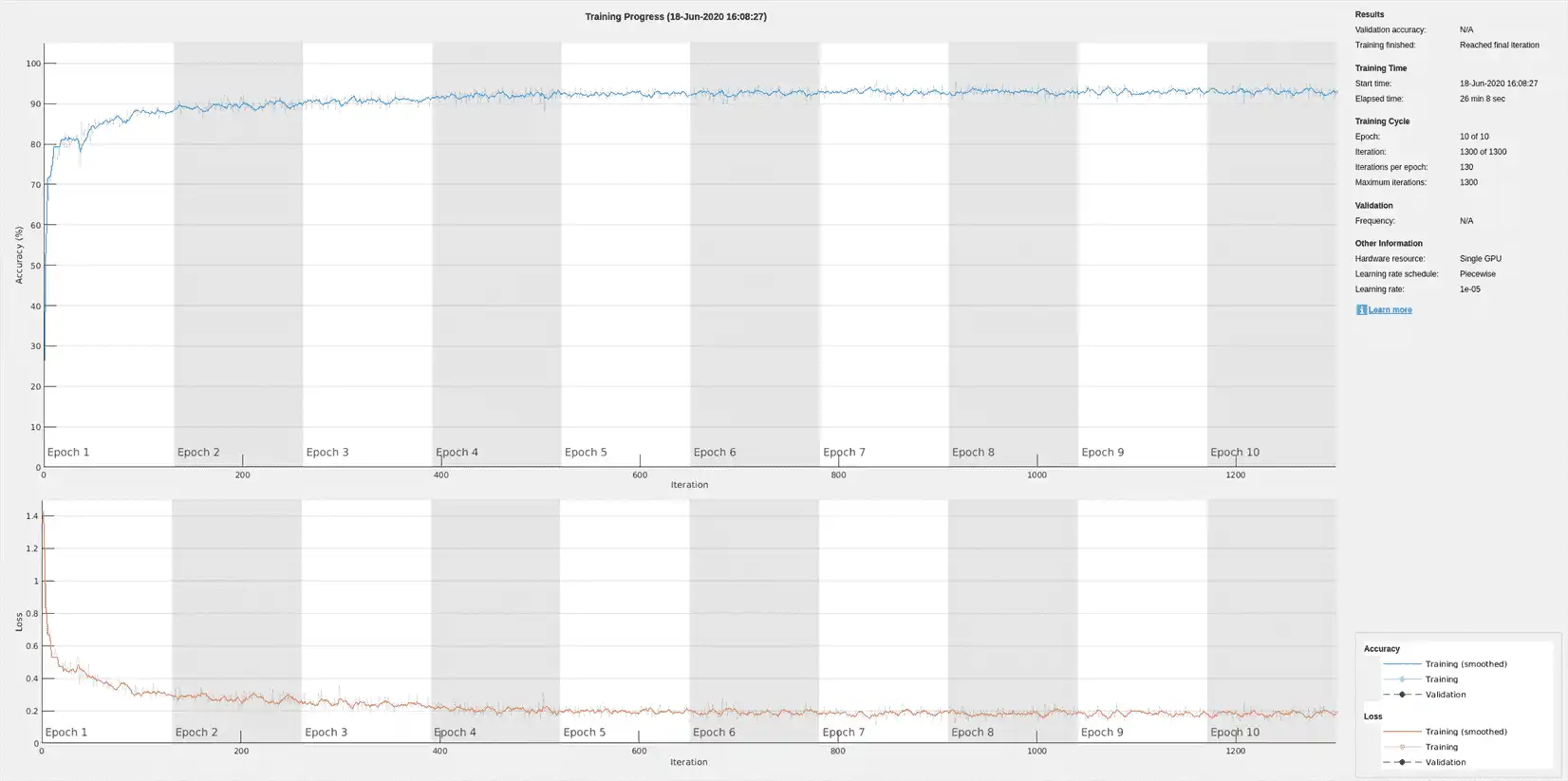
Train Network

Use the trainNetwork command to train the LSTM network.

if actionFlag == "Train networks"
     rawNet = trainNetwork(trainData(:,1),trainData(:,2),layers,options);
end

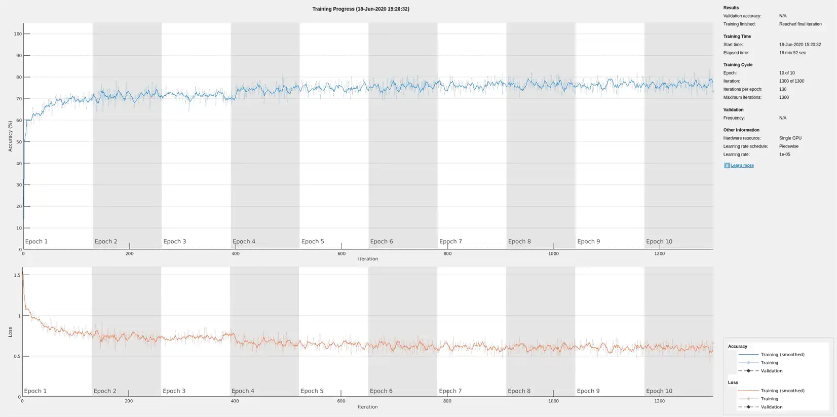
The training accuracy and loss subplots in the figure track the training progress across all iterations. Using the raw signal data, the network correctly classifies about 77% of the samples as belonging to a P wave, a QRS complex, a T wave, or an unlabeled region "n/a".

Classify Testing Data

Classify the testing data using the trained LSTM network and the classify command. Specify a mini-batch size of 50 to match the training options.

predTest = classify(rawNet,testData(:,1),'MiniBatchSize',50);

A confusion matrix provides an intuitive and informative means to visualize classification performance. Use the confusionchart command to calculate the overall classification accuracy for the testing data predictions. For each input, convert the cell array of categorical labels to a row vector. Specify a column-normalized display to view results as percentages of samples for each class.

confusionchart([predTest{:}],[testData{:,2}],'Normalization','column-normalized');

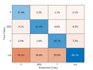
Using the raw ECG signal as input to the network, only about 60% of T-wave samples, 40% of P-wave samples, and 60% of QRS-complex samples were correct. To improve performance, apply some knowledge of the ECG signal characteristics prior to input to the deep learning network, for instance the baseline wandering caused by a patient's respiratory motion.

Apply Filtering Methods to Remove Baseline Wander and High-Frequency Noise

The three beat morphologies occupy different frequency bands. The spectrum of the QRS complex typically has a center frequency around 10–25 Hz, and its components lie below 40 Hz. The P and T waves occur at even lower frequencies: P-wave components are below 20 Hz, and T-wave components are below 10 Hz [5].

Baseline wander is a low-frequency (< 0.5 Hz) oscillation caused by the patient's breathing motion. This oscillation is independent from the beat morphologies and does not provide meaningful information [6].

Design a bandpass filter with passband frequency range of [0.5, 40] Hz to remove the wander and any high frequency noise. Removing these components improves the LSTM training because the network does not learn irrelevant features. Use cellfun on the tall data cell arrays to filter the dataset in parallel.

% Bandpass filter design
hFilt = designfilt('bandpassiir', 'StopbandFrequency1',0.4215,'PassbandFrequency1', 0.5, ...
    'PassbandFrequency2',40,'StopbandFrequency2',53.345,...
    'StopbandAttenuation1',60,'PassbandRipple',0.1,'StopbandAttenuation2',60,...
    'SampleRate',250,'DesignMethod','ellip');

% Create tall arrays from the transformed datastores and filter the signals
tallTrainSet = tall(trainDs);
tallTestSet = tall(testDs);

filteredTrainSignals = gather(cellfun(@(x)filter(hFilt,x),tallTrainSet(:,1),'UniformOutput',false));

Evaluating tall expression using the Parallel Pool 'local':
- Pass 1 of 1: 0% complete
Evaluation 0% complete

- Pass 1 of 1: Completed in 13 sec
Evaluation completed in 14 sec

trainLabels = gather(tallTrainSet(:,2));

Evaluating tall expression using the Parallel Pool 'local':
- Pass 1 of 1: Completed in 3.6 sec
Evaluation completed in 4 sec

filteredTestSignals = gather(cellfun(@(x)filter(hFilt,x),tallTestSet(:,1),'UniformOutput',false));

Evaluating tall expression using the Parallel Pool 'local':
- Pass 1 of 1: Completed in 2.4 sec
Evaluation completed in 2.5 sec

testLabels = gather(tallTestSet(:,2));

Evaluating tall expression using the Parallel Pool 'local':
- Pass 1 of 1: Completed in 1.9 sec
Evaluation completed in 2 sec

Plot the raw and filtered signals for a typical case.

trainData = gather(tallTrainSet);

Evaluating tall expression using the Parallel Pool 'local':
- Pass 1 of 1: Completed in 4 sec
Evaluation completed in 4.2 sec

figure
subplot(2,1,1)
plot(trainData{95,1}(2001:3000))
title('Raw')
grid
subplot(2,1,2)
plot(filteredTrainSignals{95}(2001:3000))
title('Filtered')
grid

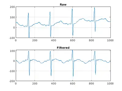
Even though the baseline of the filtered signals may confuse a physician that is used to traditional ECG measurements on medical devices, the network will actually benefit from the wandering removal.

Train Network with Filtered ECG Signals

Train the LSTM network on the filtered ECG signals using the same network architecture as before.

if actionFlag == "Train networks"
    filteredNet = trainNetwork(filteredTrainSignals,trainLabels,layers,options);
end

Preprocessing the signals improves the training accuracy to better than 80%.

Classify Filtered ECG Signals

Classify the preprocessed test data with the updated LSTM network.

predFilteredTest = classify(filteredNet,filteredTestSignals,'MiniBatchSize',50);

Visualize the classification performance as a confusion matrix.

figure
confusionchart([predFilteredTest{:}],[testLabels{:}],'Normalization','column-normalized');

Simple preprocessing improves T-wave classification by about 15%, and QRS-complex and P-wave classification by about 10%.

Time-Frequency Representation of ECG Signals

A common approach for successful classification of time-series data is to extract time-frequency features and feed them to the network instead of the original data. The network then learns patterns across time and frequency simultaneously [7].

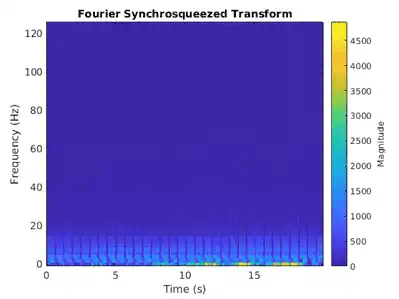
The Fourier synchrosqueezed transform (FSST) computes a frequency spectrum for each signal sample so it is ideal for the segmentation problem at hand where we need to maintain the same time resolution as the original signals. Use the fsst function to inspect the transform of one of the training signals. Specify a Kaiser window of length 128 to provide adequate frequency resolution.

data =  preview(trainDs);
figure
fsst(data{1,1},250,kaiser(128),'yaxis')

Calculate the FSST of each signal in the training dataset over the frequency range of interest, [0.5, 40] Hz. Treat the real and imaginary parts of the FSST as separate features and feed both components into the network. Furthermore, standardize the training features by subtracting the mean and dividing by the standard deviation. Use a transformed datastore, the extractFSSTFeatures helper function, and the tall function to process the data in parallel.

fsstTrainDs = transform(trainDs,@(x)extractFSSTFeatures(x,250));
fsstTallTrainSet = tall(fsstTrainDs);
fsstTrainData = gather(fsstTallTrainSet);

Evaluating tall expression using the Parallel Pool 'local':
- Pass 1 of 1: 0% complete
Evaluation 0% complete

- Pass 1 of 1: Completed in 2 min 35 sec
Evaluation completed in 2 min 35 sec

Repeat this procedure for the testing data.

fsstTTestDs = transform(testDs,@(x)extractFSSTFeatures(x,250));
fsstTallTestSet = tall(fsstTTestDs);
fsstTestData = gather(fsstTallTestSet);

Evaluating tall expression using the Parallel Pool 'local':
- Pass 1 of 1: Completed in 1 min 4 sec
Evaluation completed in 1 min 4 sec

Adjust Network Architecture

Modify the LSTM architecture so that the network accepts a frequency spectrum for each sample instead of a single value. Inspect the size of the FSST to see the number of frequencies.

size(fsstTrainData{1,1})

ans = 1×2

          40        5000

Specify a sequenceInputLayer of 40 input features. Keep the rest of the network parameters unchanged.

layers = [ ...
    sequenceInputLayer(40)
    lstmLayer(200,'OutputMode','sequence')
    fullyConnectedLayer(4)
    softmaxLayer
    classificationLayer];

Train Network with FSST of ECG Signals

Train the updated LSTM network with the transformed dataset.

if actionFlag == "Train networks"
    fsstNet = trainNetwork(fsstTrainData(:,1),fsstTrainData(:,2),layers,options);
end

Using time-frequency features improves the training accuracy, which now exceeds 90%.

Classify Test Data with FSST

Using the updated LSTM network and extracted FSST features, classify the testing data.

predFsstTest = classify(fsstNet,fsstTestData(:,1),'MiniBatchSize',50);

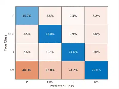
Visualize the classification performance as a confusion matrix.

confusionchart([predFsstTest{:}],[fsstTestData{:,2}],'Normalization','column-normalized');

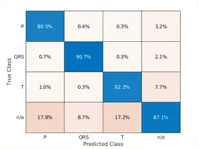
Using a time-frequency representation improves T-wave classification by about 25%, P-wave classification by about 40%, and QRS-complex classification by 30%, when compared to the raw data results.

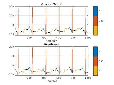
Use a signalMask object to compare the network prediction to the ground truth labels for a single ECG signal. Ignore the "n/a" labels when plotting the regions of interest.

testData = gather(tall(testDs));

Evaluating tall expression using the Parallel Pool 'local':
- Pass 1 of 1: 0% complete
Evaluation 0% complete

- Pass 1 of 1: Completed in 37 sec
Evaluation completed in 37 sec

Mtest = signalMask(testData{1,2}(3000:4000));
Mtest.SpecifySelectedCategories = true;
Mtest.SelectedCategories = find(Mtest.Categories ~= "n/a");

figure
subplot(2,1,1)
plotsigroi(Mtest,testData{1,1}(3000:4000))
title('Ground Truth')

Mpred = signalMask(predFsstTest{1}(3000:4000));
Mpred.SpecifySelectedCategories = true;
Mpred.SelectedCategories = find(Mpred.Categories ~= "n/a");

subplot(2,1,2)
plotsigroi(Mpred,testData{1,1}(3000:4000))
title('Predicted')

Conclusion

This example showed how signal preprocessing and time-frequency analysis can improve LSTM waveform segmentation performance. Bandpass filtering and Fourier-based synchrosqueezing result in an average improvement across all output classes from 55% to around 85%.