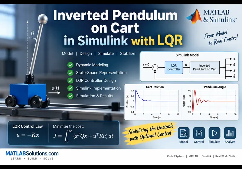
What is Inverted Pendulum on a Cart in Simulink State-Space Derivation LQR Tuning and Non-Linear Simulation?
Inverted Pendulum on a Cart in Simulink State-Space Derivation LQR Tuning and Non-Linear Simulation is a MATLAB-based technical project and simulation model. The inverted pendulum on a cart is one of the most common lab assignments in undergraduate control systems courses, including Purdue ME 475, Michigan EECS 460, and UC Berkeley EECS 128. It is an underactuated system: you have only one motor pushing the cart back and forth, but you need to control two things at once (the position of the cart and the angle of the pole balanced on top of it). A standard single-loop PID controller usually fails here because balancing the upright pole forces the cart to drift off the track. Linear Quadratic Regulator (LQR) control solves this by looking at all system states together (position, velocity, angle, and angular velocity) and calculating the exact motor force needed to keep the stick upright while bringing the cart to a commanded position. This project provides the full mathematical derivation, the parameter initialization script in MATLAB, and a complete non-linear Simulink model with motor force limits and external disturbance testing. What is included: Complete equations of motion, linearized state-space matrices, Bryson's rule tuning for Q and R matrices, and the working Simulink model (.slx) with pre-wired scopes.
Project Methodology
1. Equations of Motion
The system consists of a cart of mass M pushed by an input force u, and a pendulum of mass m, length 2*l, and moment of inertia I. Friction between the cart wheels and the ground is modeled as a damping constant b.
Using Euler-Lagrange equations, the two coupled non-linear equations for the cart acceleration and pendulum angular acceleration are:
(M + m)*x_ddot + b*x_dot + m*l*theta_ddot*cos(theta) - m*l*(theta_dot^2)*sin(theta) = u
(I + m*l^2)*theta_ddot + m*g*l*sin(theta) + m*l*x_ddot*cos(theta) = 0
2. State-Space Representation
To design an LQR controller, we define the state vector as four variables:
- x1: Cart position (meters)
- x2: Cart velocity (meters per second)
- x3: Pendulum angle deviation from upright (radians, where 0 is balanced)
- x4: Pendulum angular velocity (radians per second)
Assuming small angle deviations near the upright position, we approximate sin(theta) as theta, cos(theta) as 1, and drop the squared angular velocity terms. Setting D = I*(M + m) + M*m*l^2, the linear state-space matrices are:
A = [ 0,  1,              0,             0;
      0, -(I + m*l^2)*b/D, (m^2*g*l^2)/D, 0;
      0,  0,              0,             1;
      0, -(m*l*b)/D,       m*g*l*(M+m)/D, 0 ];

B = [ 0;
     (I + m*l^2)/D;
      0;
     (m*l)/D ];

C = eye(4);
D_matrix = zeros(4, 1);
3. Tuning the LQR Weights (Bryson's Rule)
The LQR algorithm finds the optimal feedback gain matrix K that minimizes the trade-off between keeping states near zero and not overloading the motor:
Cost = Integral of ( x'*Q*x + u'*R*u ) dt
Instead of guessing values for Q and R, we use Bryson's rule. We set each diagonal element of Q to 1 divided by the square of the maximum acceptable error for that state:
- Max cart position error: 0.1 m, so Q(1,1) = 1 / (0.1)^2 = 100
- Cart velocity weight: Q(2,2) = 1
- Max pendulum angle tilt: 0.07 rad (about 4 degrees), so Q(3,3) = 1 / (0.07)^2 = 200
- Pendulum angular velocity weight: Q(4,4) = 1
- Control effort penalty: R = 0.01 (prevents demanding more than 25 N from the motor)
4. MATLAB Setup Script (init_pendulum_params.m)
Run this script before starting the Simulink model. It loads the physical constants, checks that the system is controllable, computes gain K, and calculates the feedforward tracking gain Nbar.
% Physical parameters
M = 0.5;      % Cart mass (kg)
m = 0.2;      % Pendulum mass (kg)
b = 0.1;      % Friction coefficient (N*s/m)
l = 0.3;      % Distance to center of mass (m)
I = 0.006;    % Pendulum moment of inertia (kg*m^2)
g = 9.81;     % Gravity (m/s^2)

Den = I*(M + m) + M*m*l^2;

A = [0, 1, 0, 0;
     0, -(I + m*l^2)*b/Den, (m^2*g*l^2)/Den, 0;
     0, 0, 0, 1;
     0, -(m*l*b)/Den, m*g*l*(M + m)/Den, 0];

B = [0; (I + m*l^2)/Den; 0; (m*l)/Den];

% Check controllability
Co = ctrb(A, B);
if rank(Co) == 4
    disp('System is controllable.');
end

% LQR Weighting matrices
Q = diag([100, 1, 200, 1]);
R = 0.01;

% Calculate optimal gain K
K = lqr(A, B, Q, R);

% Calculate feedforward gain Nbar for zero steady-state position error
s = size(A, 1);
Z = [zeros(1, s) 1];
N = [A, B; [1 0 0 0], 0] \ Z';
Nbar = N(1+s) + K * N(1:s);
5. Simulink Model Structure
The companion Simulink file (inverted_pendulum_nonlinear.slx) runs the full non-linear model rather than the simplified linear version. Key blocks include:
- Non-Linear Dynamics Subsystem: Uses Integrator, Trigonometric, and Math Function blocks to evaluate the exact equations without small-angle assumptions.
- Motor Force Saturation: A Saturation block caps the control force at plus/minus 25 N to reflect real motor limits.
- Impulse Disturbance: A pulse generator adds a 5 N force pulse for 0.2 seconds at t = 5 s, simulating someone tapping the cart.
- Pre-Wired Scopes: Scopes track cart position against the setpoint, pendulum tilt angle, and the required motor force.
6. Simulation Results
| Test Metric | Open-Loop (No Control) | Closed-Loop LQR Control |
|---|---|---|
| System Stability | Unstable pole at +5.56 | All poles in left-half plane |
| Pendulum Settling Time | Falls over within 0.4 s |
Verified MATLAB Simulation Code Demonstration
Syntax-highlighted executable code demonstration for Inverted Pendulum on a Cart in Simulink State-Space Derivation LQR Tuning and Non-Linear Simulation:
% State-Space Control & Stability Analysis
clc; clear; close all;

% System Matrices
A = [0 1; -4 -5];
B = [0; 1];
C = [1 0];
D = 0;

sys_ss = ss(A, B, C, D);
Co = ctrb(A, B);

% Pole Placement Control
desired_poles = [-3 + 4i, -3 - 4i];
K = acker(A, B, desired_poles);

sys_cl = ss(A - B*K, B, C, D);
fprintf('State Feedback Controller Formulated Successfully!\n');