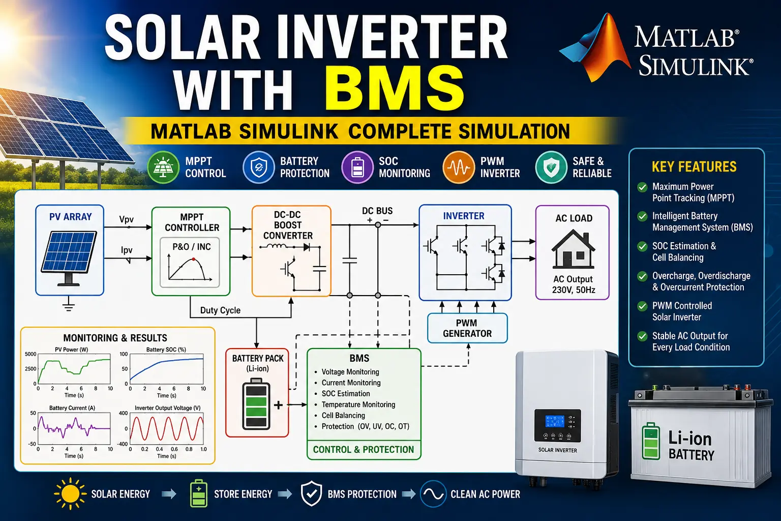
What is Solar Inverter with BMS in MATLAB Simulink Complete Simulation Project?
Solar Inverter with BMS in MATLAB Simulink Complete Simulation Project is a MATLAB-based technical project and simulation model. Modern solar energy systems combine photovoltaic (PV) generation with integrated battery energy storage to supply reliable residential and commercial power, provide emergency backup during grid blackouts, and reduce peak electricity charges. A complete solar inverter system with an integrated Battery Management System (BMS) comprises three interdependent power stages: an MPPT DC-DC boost converter to track peak solar irradiance, a bidirectional DC-DC converter for controlled battery charging and discharging, and a Voltage Source Inverter (VSI) to supply clean sinusoidal AC power to local appliances or the utility grid. In MATLAB and Simulink, using Simscape Electrical allows engineers to simulate semiconductor switching dynamics, design cascaded feedback controllers, monitor battery state-of-charge (SoC) protection limits, and ensure compliance with IEEE 1547 grid interconnection standards. This project covers the architectural modeling, BMS control logic, inverter modulation, and dynamic closed-loop simulation of a complete solar inverter with battery storage in MATLAB.
Project Methodology
The design, control architecture, and dynamic simulation of a solar inverter with an integrated BMS in MATLAB Simulink follows a structured power electronics and energy storage workflow:
- Solar PV Array & MPPT Boost Converter Modeling: Configure a solar PV array module in Simscape Electrical, characterizing non-linear P-V and I-V curves across varying irradiance (200 W/m² to 1000 W/m²). Design a DC-DC boost converter driven by a Perturb and Observe (P&O) MPPT algorithm to extract peak solar power.
- Lithium-Ion Battery Storage & BMS Setup:
- Model a Lithium-Ion battery pack with dynamic equivalent circuit parameters and open-circuit voltage tracking.
- Implement a Battery Management System (BMS) in MATLAB to execute real-time State-of-Charge (SoC) estimation, overcharge protection (capping charge at 90% SoC), deep-discharge prevention (disconnecting discharge below 20% SoC), and current limiting.
- Bidirectional DC-DC Converter & DC Bus Control: Interface the battery pack with the common 400V DC bus via a bidirectional buck-boost converter, designing dual-loop PI controllers to execute Constant Current and Constant Voltage (CC-CV) charging regimes.
- Inverter Power Stage & LCL Filter Sizing: Build a full-bridge Voltage Source Inverter (VSI) in Simscape Electrical, sizing an LCL output filter to attenuate high-frequency switching harmonics and deliver smooth sinusoidal output currents.
- Inverter Closed-Loop Modulation & Grid Synchronization:
- Implement a Phase-Locked Loop (PLL) for phase angle detection at the Point of Common Coupling (PCC).
- Design decoupled synchronous d-q frame PI current controllers to govern active power export and maintain unity power factor.
- Incorporate autonomous voltage-frequency (V-f) regulation mode to power critical AC loads during grid outages (islanding mode).
- Supervisory Energy Management System (EMS): Program state-machine control logic in Stateflow to govern multi-mode power routing:
- Directing solar generation to meet immediate AC load demand.
- Routing surplus solar energy to recharge the battery bank.
- Discharging the battery to support AC loads during cloud cover or night hours.
- Exporting excess clean power to the utility grid once the battery reaches full charge.
- Dynamic Simulation & Power Quality Validation: Simulate the integrated system in MATLAB Simulink across sharp solar irradiance transitions and sudden AC load steps, evaluating DC bus voltage stability (±2%), battery SoC tracking, and AC current Total Harmonic Distortion (THD < 5%) compliant with IEEE 1547 standards.
Verified MATLAB Simulation Code Demonstration
Syntax-highlighted executable code demonstration for Solar Inverter with BMS in MATLAB Simulink Complete Simulation Project:
% Dynamic Physical Model & Solver Configuration
clc; clear; close all;

% Hydraulic & Mechanical ODE System Parameters
m = 1.0; c = 0.5; k = 9.0;
ode_sys = @(t, y) [y(2); -(c/m)*y(2) - (k/m)*y(1)];

% Numerical ODE Integration
tspan = [0 10]; y0 = [1.0; 0.0];
[t, y] = ode45(ode_sys, tspan, y0);

fprintf('ODE Physical System Solved across %d Time Steps!\n', length(t));