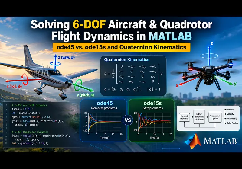
Simulating a 6-Degree-of-Freedom (6-DOF) flight vehicle in MATLAB looks straightforward on paper. You set up Newton-Euler equations of motion, calculate aerodynamic forces, and pass the state vector to a numerical solver. In practice, flight dynamics projects run into two frequent issues: kinematic singularities from Euler angles and simulation stalls where ode45 slows down to an unusable crawl.
Whether you are modeling a fixed-wing UAV or a multirotor drone, resolving these issues requires moving to quaternion kinematics and selecting the right numerical solver for stiff system dynamics.
1. The Gimbal Lock Problem: Why Euler Angles Fail
Introductory flight mechanics courses usually define vehicle attitude with Euler angles: roll (phi), pitch (theta), and yaw (psi). The kinematic equation relating body angular rates [p, q, r] to Euler angle rates relies on a transformation matrix containing tan(theta) and 1/cos(theta) terms:
[ dphi/dt   ]   [ 1   sin(phi)*tan(theta)   cos(phi)*tan(theta) ] [ p ]
[ dtheta/dt ] = [ 0   cos(phi)             -sin(phi)            ] [ q ]
[ dpsi/dt   ]   [ 0   sin(phi)/cos(theta)   cos(phi)/cos(theta) ] [ r ]
When an aircraft climbs steeply, enters a dive, or a quadrotor pitches aggressively past 85 degrees, cos(theta) approaches zero. The tangent term spikes toward infinity, triggering divide-by-zero errors in MATLAB.
Unit Quaternions as an Alternative
Quaternions represent orientation as a four-element vector, q = [q0, q1, q2, q3], describing a rotation around an arbitrary axis. The rate of change of the quaternion attitude is calculated through a linear matrix multiplication:
dq/dt = 0.5 * Omega(omega) * qThis formulation eliminates trigonometric division entirely. However, numerical integration introduces truncation error over time, causing the norm of q to drift away from 1. If your code does not normalize the quaternion at each time step, the attitude solution will gradually drift or diverge.
2. Solver Selection: Why ode45 Stalls and When to Use ode15s
Most engineering students default to ode45 (explicit Runge-Kutta) for every simulation. For an uncoupled rigid body, ode45 works well. But real 6-DOF flight models combine fast and slow dynamics:
- Fast dynamics: Motor electrical time constants (5 to 15 milliseconds), propeller inertia, and rapid aerodynamic damping.
- Slow dynamics: Phugoid trajectory oscillations and position tracking over seconds or minutes.
This separation of time scales creates numerical stiffness. When ode45 encounters a stiff system, its adaptive step-size algorithm reduces the time step below 1e-7 seconds to maintain stability. The simulation appears frozen, taking hours to compute a few seconds of flight time.
When to switch to ode15s
ode15s is an implicit, variable-order solver based on numerical differentiation formulas. It handles stiff systems by evaluating the Jacobian, allowing it to take larger time steps without losing stability. If your 6-DOF model includes motor lags, high-gain attitude controllers, or stiff control surfaces, ode15s is often 10 to 50 times faster than ode45.
3. Methods and Solvers Compared
| Method or Solver | Best Suited For | Primary Limitation | Failure Mode |
|---|---|---|---|
| Euler Angles | Level cruising flight with pitch below 60 degrees | Kinematic singularity at +/- 90 degrees pitch | Division by zero and NaN states |
| Quaternions | Full 3D aerobatic maneuvers and quadrotor flips | Requires unit-norm constraint enforcement | Norm drift corrupts rotational kinematics |
| ode45 | Non-stiff rigid body dynamic models | Stalls when fast actuator time constants are added | Step-size collapse; simulation freezes |
| ode15s | Coupled motor dynamics and stiff aerodynamic equations | Jacobian computation overhead | Slightly slower on purely non-stiff systems |
Closing the Loop on Your Flight Simulation
Setting up theoretical equations is only part of the task. A working flight simulation requires:
- Stability and control derivatives (CL_alpha, Cmq, Cn_beta, Clp).
- Propeller thrust curves and motor lag models.
- Quaternion normalization and conversion back to Euler angles for plotting.
- Inner attitude and outer position control loops.
If your simulation is diverging, running slowly, or failing course benchmarks, our engineering team can review your equations, calibrate your stability matrices, and verify your MATLAB scripts and Simulink models.
Need Verified Flight Dynamics and Control Assistance?
Explore our reference models or connect directly with an aerospace engineering mentor:
Browse Control Systems Projects Simulink Modeling HelpExecutable MATLAB Script & Model Setup
% =========================================================================
% 6-DOF FLIGHT DYNAMICS STATE PROPAGATOR SKELETON
% Framework: Quaternion Kinematics and Newton-Euler Rigid Body Dynamics
% Solvers: ode45 (Non-stiff) vs. ode15s (Stiff actuator coupling)
% =========================================================================
function flight_dynamics_demo()
    clear; clc; close all;

    % --- Initial Conditions ---
    % State Vector X: [u; v; w; p; q; r; q0; q1; q2; q3; x; y; z]
    V_init = [15; 0; 0];          % Body translational velocities (m/s)
    omega_init = [0; 0; 0];       % Body angular rates (rad/s)
    q_init = [1; 0; 0; 0];        % Initial attitude quaternion (level flight)
    pos_init = [0; 0; -100];      % Position in NED frame (m)

    X0 = [V_init; omega_init; q_init; pos_init];
    tspan = [0 10];               % Simulation horizon (seconds)

    % --- Solver Execution ---
    % Note: Use ode15s if incorporating stiff motor/ESC dynamics
    options = odeset('RelTol', 1e-5, 'AbsTol', 1e-7);

    fprintf('Integrating 6-DOF equations of motion...\n');
    [t, X] = ode45(@(t, x) derivatives_6dof(t, x), tspan, X0, options);

    % Plot altitude profile
    figure('Color', 'w');
    plot(t, -X(:, 12), 'b-', 'LineWidth', 1.5);
    grid on; xlabel('Time (s)'); ylabel('Altitude (m)');
    title('6-DOF Altitude Trajectory (NED Frame)');
end

% --- Equations of Motion Derivative Function ---
function dX = derivatives_6dof(t, X)
    % Unpack State Vector
    u = X(1); v = X(2); w = X(3);
    p = X(4); q = X(5); r = X(6);
    q_att = X(7:10); % [q0, q1, q2, q3]

    % Physical Constants and Mass Properties
    m = 1.5; % Mass (kg)
    % Inertia Tensor (kg*m^2)
    Ixx = 0.03; Iyy = 0.03; Izz = 0.05;
    I = diag([Ixx, Iyy, Izz]);

    omega = [p; q; r];

    % 1. Applied Forces and Moments (Body Frame)
    % TODO: Replace with full stability derivatives or quadrotor mixer matrix
    % Aerodynamic lift, drag, and thrust coupling:
    Total_Forces = [1.5 * 9.81; 0; -m * 9.81]; % [Fx; Fy; Fz]
    Total_Moments = [0.01 * sin(t); 0.005; 0]; % [Mx; My; Mz]

    % 2. Translational Dynamics (Body Frame Newton's Second Law)
    % du/dt = F/m - cross(omega, V)
    V_dot = (Total_Forces / m) - cross(omega, [u; v; w]);

    % 3. Rotational Dynamics (Euler's Rotational Equations)
    % I * domega/dt = M - cross(omega, I * omega)
    omega_dot = I \ (Total_Moments - cross(omega, I * omega));

    % 4. Quaternion Attitude Kinematics (Singularity-Free)
    Omega_matrix = [
         0, -p, -q, -r;
         p,  0,  r, -q;
         q, -r,  0,  p;
         r,  q, -p,  0
    ];
    q_dot = 0.5 * Omega_matrix * q_att;

    % TODO: Implement continuous Baumgarte stabilization or normalization
    % to prevent numerical quaternion norm drift (|q| != 1) over long runs

    % 5. Navigation Kinematics (Body to NED Earth Frame)
    % TODO: Convert quaternion to Direction Cosine Matrix (DCM)
    % and project [u, v, w] into Earth NED coordinates [x_dot, y_dot, z_dot]
    pos_dot = [u; v; w]; % Simplified dummy mapping

    dX = [V_dot; omega_dot; q_dot; pos_dot];
endRelated Verified MATLAB & Simulink Projects
Need pre-built, debugged Simulink models with complete parameter initialization scripts and documentation? Explore top related solutions:
Common Engineering Troubleshooting & Q&A
Frequently encountered bugs, solver convergence issues, and implementation questions answered by our engineering mentors:
Recommended Engineering Articles
Need Custom MATLAB / Simulink Implementation?
Our team of PhD engineers build custom simulation plants, train machine learning agents, tune PID/MPC controllers, and deliver complete, executable code with Turnitin reports.