Linear Regression 2

Model Display

A linear regression model shows several diagnostics when you enter its name or enter disp(mdl). This display gives some of the basic information to check whether the fitted model represents the data adequately.

For example, fit a linear model to data constructed with two out of five predictors not present and with no intercept term:

X = randn(100,5);
y = X*[1;0;3;0;-1] + randn(100,1);
mdl = fitlm(X,y)

mdl = 
Linear regression model:
    y ~ 1 + x1 + x2 + x3 + x4 + x5

Estimated Coefficients:
                   Estimate        SE        tStat        pValue  
                   _________    ________    ________    __________

    (Intercept)     0.038164    0.099458     0.38372       0.70205
    x1               0.92794    0.087307      10.628    8.5494e-18
    x2             -0.075593     0.10044    -0.75264       0.45355
    x3                2.8965    0.099879          29    1.1117e-48
    x4              0.045311     0.10832     0.41831       0.67667
    x5              -0.99708     0.11799     -8.4504     3.593e-13


Number of observations: 100, Error degrees of freedom: 94
Root Mean Squared Error: 0.972
R-squared: 0.93,  Adjusted R-Squared: 0.926
F-statistic vs. constant model: 248, p-value = 1.5e-52

Notice that:

ANOVA

To examine the quality of the fitted model, consult an ANOVA table. For example, use anova on a linear model with five predictors:

tbl = anova(mdl)

tbl=6×5 table
              SumSq     DF    MeanSq        F         pValue  
             _______    __    _______    _______    __________

    x1        106.62     1     106.62     112.96    8.5494e-18
    x2       0.53464     1    0.53464    0.56646       0.45355
    x3        793.74     1     793.74     840.98    1.1117e-48
    x4       0.16515     1    0.16515    0.17498       0.67667
    x5        67.398     1     67.398      71.41     3.593e-13
    Error     88.719    94    0.94382                         

This table gives somewhat different results than the model display. The table clearly shows that the effects of x2 and x4 are not significant. Depending on your goals, consider removing x2 and x4 from the model.

Diagnostic Plots

Diagnostic plots help you identify outliers, and see other problems in your model or fit. For example, load the carsmall data, and make a model of MPG as a function of Cylinders (categorical) and Weight:

load carsmall
tbl = table(Weight,MPG,Cylinders);
tbl.Cylinders = categorical(tbl.Cylinders);
mdl = fitlm(tbl,'MPG ~ Cylinders*Weight + Weight^2');

Make a leverage plot of the data and model.

plotDiagnostics(mdl)

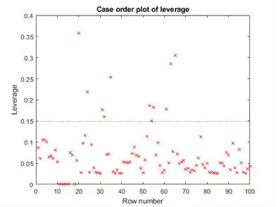
There are a few points with high leverage. But this plot does not reveal whether the high-leverage points are outliers.

Look for points with large Cook’s distance.

plotDiagnostics(mdl,'cookd')

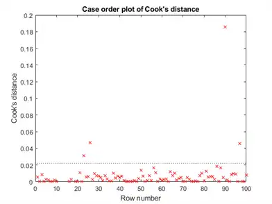
There is one point with large Cook’s distance. Identify it and remove it from the model. You can use the Data Cursor to click the outlier and identify it, or identify it programmatically:

[~,larg] = max(mdl.Diagnostics.CooksDistance);
mdl2 = fitlm(tbl,'MPG ~ Cylinders*Weight + Weight^2','Exclude',larg);

Residuals — Model Quality for Training Data

There are several residual plots to help you discover errors, outliers, or correlations in the model or data. The simplest residual plots are the default histogram plot, which shows the range of the residuals and their frequencies, and the probability plot, which shows how the distribution of the residuals compares to a normal distribution with matched variance.

Examine the residuals:

plotResiduals(mdl)

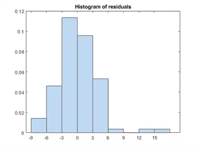
The observations above 12 are potential outliers.

plotResiduals(mdl,'probability')

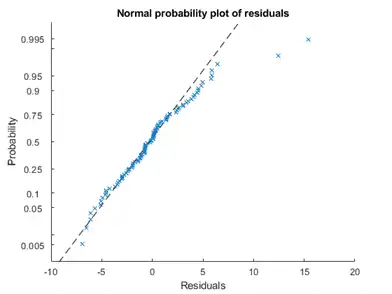
The two potential outliers appear on this plot as well. Otherwise, the probability plot seems reasonably straight, meaning a reasonable fit to normally distributed residuals.

You can identify the two outliers and remove them from the data:

outl = find(mdl.Residuals.Raw > 12)

outl = 2×1

    90
    97

To remove the outliers, use the Exclude name-value pair:

mdl3 = fitlm(tbl,'MPG ~ Cylinders*Weight + Weight^2','Exclude',outl);

Examine a residuals plot of mdl2: