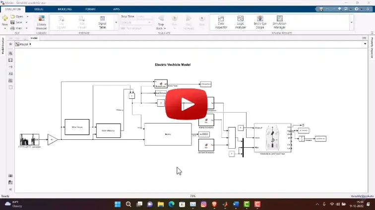
What is Electric Car Simulation in MATLAB: Complete Modeling Guide?
Electric Car Simulation in MATLAB: Complete Modeling Guide is a MATLAB-based technical project and simulation model. Electric vehicle (EV) development relies heavily on model-based design to size battery packs, select traction motors, and test energy management strategies before building physical prototypes. Testing how an EV handles steep grades, highway cruising, and stop-and-go city traffic in software helps automotive engineers optimize vehicle range and battery lifespan early in the design cycle. Simulating an electric car requires capturing interactions across multiple engineering domains: longitudinal vehicle dynamics, electrical battery behavior, motor electromagnetics, power inverter switching, and mechanical gear transmission. Using MATLAB, Simulink, and tools like the Powertrain Blockset or Simscape Driveline, engineers can build full virtual vehicle models. These models allow developers to run standard regulatory drive cycles (such as WLTP or FTP-75), track real-time battery drain, evaluate motor torque limits, and test regenerative braking strategies under repeatable driving conditions.
Project Methodology
The electric vehicle simulation combines longitudinal body physics with electrical power flow and closed-loop motor control. The modeling process follows five practical stages:
- Drive cycle and driver model setup: Import standard speed-time drive cycles (such as the Worldwide Harmonized Light Vehicles Test Procedure (WLTP), EPA FTP-75, or custom city routes). A longitudinal driver block (typically a PI controller) compares target vehicle speed against actual speed to generate real-time throttle and brake commands.
- Vehicle chassis and aerodynamic load modeling: Calculate opposing road loads acting on the moving car using classical vehicle dynamics blocks in Simulink. The vehicle body subsystem computes aerodynamic drag, rolling resistance from tire-road contact, gravitational resistance on road inclines, and the total inertial force required for acceleration.
- Electric powertrain and motor drive modeling: Model the core electrical propulsion units:
- Traction motor: Simulate a three-phase Permanent Magnet Synchronous Motor (PMSM) or Brushless DC (BLDC) motor, including torque-speed characteristics, back-EMF, and thermal losses.
- Motor controller and inverter: Implement Field Oriented Control (FOC) or Space Vector Pulse Width Modulation (SVPWM) to convert driver torque requests into precise three-phase stator voltages.
- Transmission and differential: Model a single-speed reduction gearbox and open differential to step down motor speed and multiply torque delivered to the driven wheels.
- High-voltage battery pack and energy storage modeling: Build an equivalent circuit model (Thevenin or Rint model) of a lithium-ion battery pack. The model tracks battery terminal voltage, internal resistance, state of charge (SOC) through Coulomb counting, open-circuit voltage curves, and cell temperature rise during aggressive acceleration bursts.
- Regenerative braking logic and drive cycle simulation: Configure the brake blending algorithm. When the driver applies the brakes, the motor acts as a generator, converting kinetic energy into electrical power to recharge the battery pack up to motor and battery current limits. Conventional friction brakes engage only when deceleration demands exceed the regenerative capacity.
After running the simulation over a full drive cycle, key performance metrics are plotted and evaluated. These include total driving range on a single charge, energy consumption in kilowatt-hours per hundred kilometers (kWh/100 km), 0 to 100 km/h acceleration times, peak motor efficiency operating points, and final battery state of charge.
Verified MATLAB Simulation Code Demonstration
Syntax-highlighted executable code demonstration for Electric Car Simulation in MATLAB: Complete Modeling Guide:
% Dynamic Physical Model & Solver Configuration
clc; clear; close all;

% Hydraulic & Mechanical ODE System Parameters
m = 1.0; c = 0.5; k = 9.0;
ode_sys = @(t, y) [y(2); -(c/m)*y(2) - (k/m)*y(1)];

% Numerical ODE Integration
tspan = [0 10]; y0 = [1.0; 0.0];
[t, y] = ode45(ode_sys, tspan, y0);

fprintf('ODE Physical System Solved across %d Time Steps!\n', length(t));