ROS 2 and MATLAB Co-Simulation for Autonomous Mobile Robot Path Tracking Using NMPC

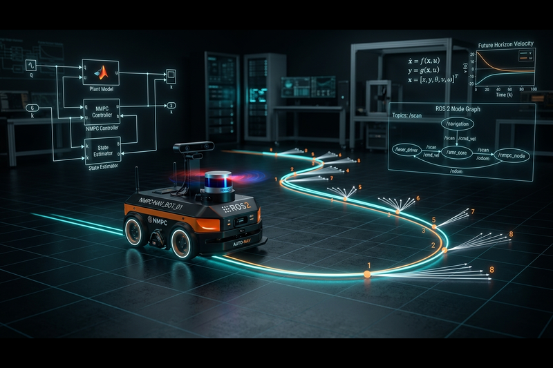
Tracking complex trajectories with non-holonomic mobile robots requires handling physical constraints such as actuator saturation, wheel slip, and sharp cornering. Standard controllers like Pure Pursuit or classic PID work well on gentle paths, but they degrade when robots operate near motor limits or encounter sudden turns.

Nonlinear Model Predictive Control (NMPC) solves a constrained optimization problem at each sampling step. It predicts future robot states over a receding time horizon and calculates optimal control commands while strictly enforcing physical limits.

This tutorial demonstrates how to build an end-to-end co-simulation pipeline between ROS 2 and MATLAB. You will configure the kinematic model of a differential drive robot, formulate the NMPC cost function, set up ROS 2 publishers and subscribers, and run closed-loop trajectory tracking.

1. Kinematic Model of a Differential Drive Robot

A standard unicycle-type differential-drive mobile robot operates in a 2D plane with state vector:

x(t) = [p_x, p_y, θ]T

where p_x and p_y represent the 2D position coordinates of the robot center, and θ is the orientation (yaw angle).

The control input vector is:

u(t) = [v, ω]T

where v is linear velocity and ω is angular velocity.

The continuous kinematic equations of motion are:

• dp_x / dt = v · cos(θ)
• dp_y / dt = v · sin(θ)
• dθ / dt = ω

Using Euler forward discretization with sampling period Ts, the discrete-time state update equations are:

• p_x(k+1) = p_x(k) + v(k) · cos(θ(k)) · Ts
• p_y(k+1) = p_y(k) + v(k) · sin(θ(k)) · Ts
• θ(k+1) = θ(k) + ω(k) · Ts

2. NMPC Problem Formulation

At each time step k, the NMPC controller solves the following optimal control problem across prediction horizon N:

min Σj=0N-1 [ ||xj - xref,j||Q2 + ||uj - uref,j||R2 ] + ||xN - xref,N||Q_N2

State and Actuator Constraints:

• Linear velocity limits: 0.0 ≤ v ≤ vmax (forward motion only)
• Angular velocity limits: -ωmax ≤ ω ≤ ωmax
• Acceleration limits: |Δv| ≤ amax · Ts
• Steering rate limits: |Δω| ≤ αmax · Ts

The state weighting matrix Q = diag(q_x, q_y, q_θ) prioritizes Cartesian path accuracy, while the input penalty matrix R = diag(r_v, r_ω) damps aggressive control actions to prevent motor saturation and wheel slip.

3. Architecture: Bridging ROS 2 and MATLAB

Communication between MATLAB and ROS 2 runs over native DDS (Data Distribution Service). MATLAB acts as a node within the ROS 2 graph, reading robot odometry, executing the sequential quadratic programming (SQP) solver, and publishing velocity commands directly back to the simulator or physical robot.

4. Implementation Steps in MATLAB

Step 1: Initialize the ROS 2 Node and Topics

Create the MATLAB ROS 2 node, subscribe to the odometry topic, and configure the velocity publisher:

ros2node_matlab = ros2node("/matlab_nmpc_node");
cmd_pub = ros2publisher(ros2node_matlab, "/cmd_vel", "geometry_msgs/Twist");
cmd_msg = ros2message(cmd_pub);
odom_sub = ros2subscriber(ros2node_matlab, "/odom", "nav_msgs/Odometry");

Step 2: Define Prediction Horizon and Weights

Set a sampling time of 0.1 s and a prediction horizon of N = 15 steps. This balances tracking fidelity with solver computation time:

Ts = 0.1;               % Sampling period (10 Hz)
N = 15;                 % Prediction horizon
Q = diag([10.0, 10.0, 1.5]);  % State weights [x, y, theta]
R = diag([0.5, 0.2]);         % Control weights [v, w]
lb = repmat([0.0; -1.2], N, 1);
ub = repmat([1.0;  1.2], N, 1);

Step 3: Execute the Real-Time Control Loop

At each iteration, parse the robot pose, solve the NMPC cost function using fmincon, apply the first control input, and publish to /cmd_vel.

5. Common Pitfalls and Engineering Solutions

1. Heading Angle Discontinuities

Heading errors can jump from +π to -π. Always normalize angular error using atan2(sin(err), cos(err)) before passing states to the solver. Without angle wrapping protection, the robot will spin erratically near the branch cut.

2. Solver Computation Time vs. Jitter

Keep the prediction horizon N between 10 and 20 steps. If the solver takes longer than the sampling period (Ts = 0.1 s), the robot will lag behind the reference trajectory. For real-time hardware execution, generate standalone C++ code using MATLAB Coder.

3. Obstacle Avoidance Feasibility

Hard distance constraints can cause the optimization solver to return infeasible status codes if the robot gets trapped. Use soft barrier functions with slack variables so the solver returns a safe braking command rather than terminating.

6. Project Support and Custom Engineering Services

Need assistance with advanced robotics controllers, custom vehicle kinematics, or ROS 2 hardware integration?

• For Students and Academic Researchers: We provide complete simulation models, thesis mentoring, and reproducible benchmark code.
• For Engineering Teams and Companies: We design custom NMPC path planners, Embedded Coder deployment pipelines, and Hardware-in-the-Loop (HIL) test rigs.

Contact the MatlabSolutions engineering team to discuss your project requirements or request custom MATLAB/Simulink source code.