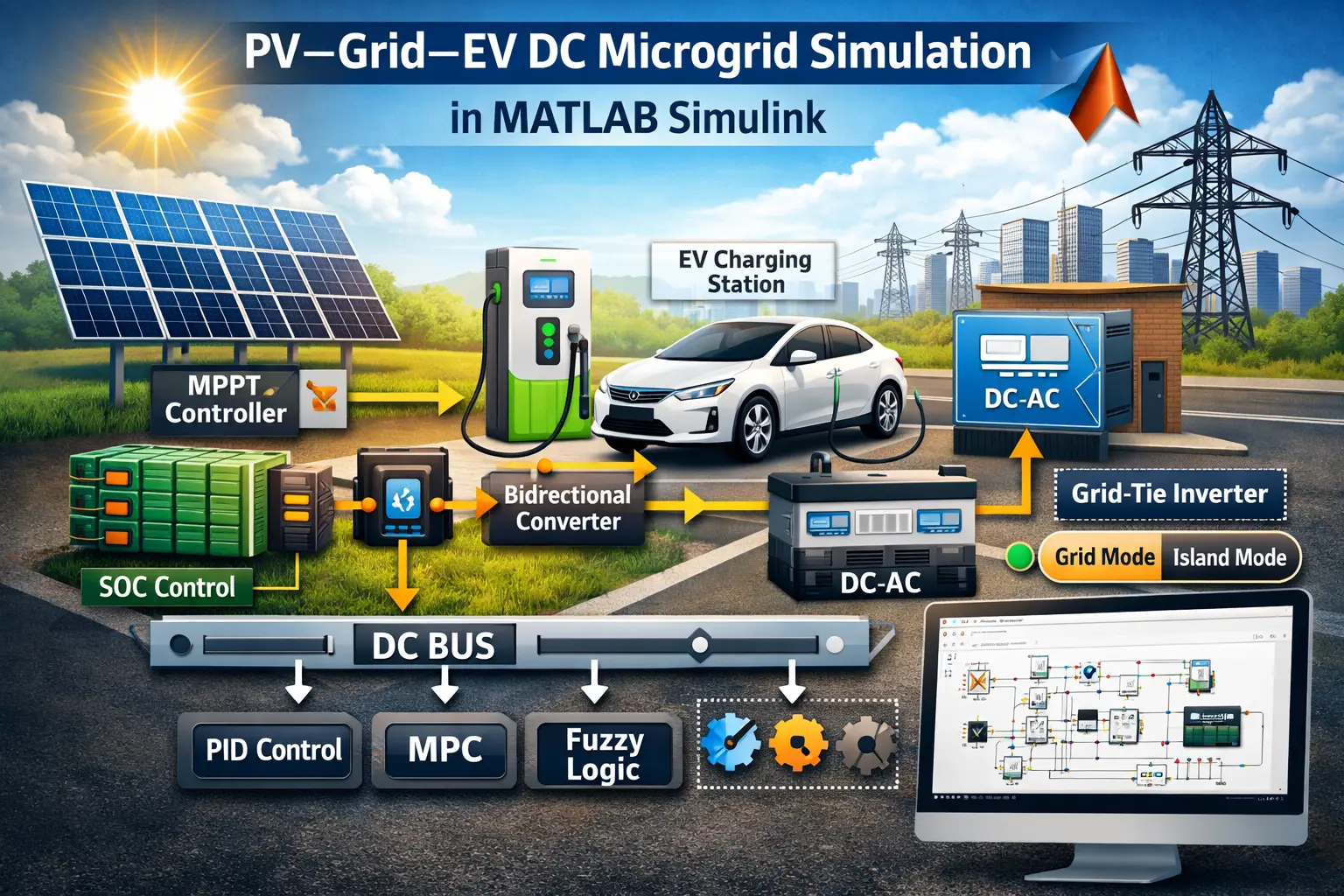
What is PV-Battery-EV DC Microgrid Simulation in MATLAB Simulink with ZVT converter?
PV-Battery-EV DC Microgrid Simulation in MATLAB Simulink with ZVT converter is a MATLAB-based technical project and simulation model. The integration of renewable energy sources, electric vehicles, and intelligent power management has become essential for modern power systems. A PV–Grid–EV DC microgrid provides an efficient architecture for combining solar photovoltaic generation, battery energy storage, and electric vehicle charging within a unified DC framework. This project focuses on the modeling and simulation of a PV–Grid–EV DC microgrid in MATLAB Simulink using Simscape Electrical. The system includes a solar PV array with MPPT control, a battery energy storage system (BESS) with state-of-charge management, EV charging infrastructure with bidirectional capability (V2G), and a grid interface for controlled power exchange.
Project Methodology
System Design: Develop a PV–Grid–EV DC microgrid architecture with a common DC bus in MATLAB Simulink (Simscape Electrical).
-
PV Modeling: Model the solar PV array with a DC–DC boost converter and implement MPPT (P&O or Incremental Conductance) for maximum power extraction.
-
Battery Integration: Implement a Battery Energy Storage System (BESS) with SOC-based charge/discharge control using a bidirectional converter.
-
EV Charging Unit: Connect the EV load to the DC bus with controlled charging (optional V2G capability).
-
Grid Interface: Design a grid-side inverter for bidirectional power exchange in grid-connected and islanded modes.
-
Control Strategy: Apply PID (or MPC/Fuzzy) control for DC bus voltage regulation and power flow management.
-
Simulation & Analysis: Test the system under varying irradiance and load conditions to evaluate voltage stability, power balance, and system performance.
Verified MATLAB Simulation Code Demonstration
Syntax-highlighted executable code demonstration for PV-Battery-EV DC Microgrid Simulation in MATLAB Simulink with ZVT converter:
% Dynamic Physical Model & Solver Configuration
clc; clear; close all;

% Hydraulic & Mechanical ODE System Parameters
m = 1.0; c = 0.5; k = 9.0;
ode_sys = @(t, y) [y(2); -(c/m)*y(2) - (k/m)*y(1)];

% Numerical ODE Integration
tspan = [0 10]; y0 = [1.0; 0.0];
[t, y] = ode45(ode_sys, tspan, y0);

fprintf('ODE Physical System Solved across %d Time Steps!\n', length(t));