Kshitij Singh answered . 2024-05-20 09:07:30

% Simulation of a projectile launched in a drag-free environment.
clc;    % Clear the command window.
close all;  % Close all figures (except those of imtool.)
clear;  % Erase all existing variables. Or clearvars if you want.
workspace;  % Make sure the workspace panel is showing.
format long g;
format compact;
fontSize = 20;

%===========================================================================================================================================================
%========== GET PARAMETERS FROM USER =======================================================================================================================
%===========================================================================================================================================================
g = -9.81;		% Acceleration due to gravity. In meters per second^2
x0 = 0;			% Lateral distance of launch site.  In meters.
y0 = 10;		% Vertical height of launch site. In meters
v0 = 16;		% Initial velocity at the angle of launch.  In meters per second.
angle = 45;		% Launch angle in degrees.

% Ask user for initial values.
defaultValue = {num2str(angle), num2str(x0), num2str(y0), num2str(v0)};
titleBar = 'Enter values';
userPrompt = {'Initial angle in degrees : ', 'Initial launch lateral distance in meters : ', 'Initial launch height in meters : ', 'Initial velocity in meters per second : '};
caUserInput = inputdlg(userPrompt, titleBar, 1, defaultValue, 'on');
if isempty(caUserInput),return,end % Bail out if they clicked Cancel.
% Convert to floating point from string.
usersValue1 = str2double(caUserInput{1});
usersValue2 = str2double(caUserInput{2});
usersValue3 = str2double(caUserInput{3});
usersValue4 = str2double(caUserInput{4});
% Check for a valid number.
if isnan(usersValue1)
    % They didn't enter a number.  
    % They clicked Cancel, or entered a character, symbols, or something else not allowed.
	% Convert the default from a string and stick that into usersValue1.
    usersValue1 = str2double(defaultValue{1});
    message = sprintf('I said it had to be a number.\nTry replacing the user.\nI will use %.2f and continue.', usersValue1);
    uiwait(warndlg(message));
end
% Do the same for usersValue2
if isnan(usersValue2)
    % They didn't enter a number.  
    % They clicked Cancel, or entered a character, symbols, or something else not allowed.
	% Convert the default from a string and stick that into usersValue1.
    usersValue2 = str2double(defaultValue{2});
    message = sprintf('I said it had to be a number.\nTry replacing the user.\nI will use %.2f and continue.', usersValue1);
    uiwait(warndlg(message));
end
if isnan(usersValue3)
    % They didn't enter a number.  
    % They clicked Cancel, or entered a character, symbols, or something else not allowed.
	% Convert the default from a string and stick that into usersValue1.
    usersValue3 = str2double(defaultValue{3});
    message = sprintf('I said it had to be a number.\nTry replacing the user.\nI will use %.2f and continue.', usersValue1);
    uiwait(warndlg(message));
end
% Assign user's values:
angle = usersValue1; % Degrees
x0 = usersValue2;
y0 = usersValue3;
v0 = usersValue4;


%===========================================================================================================================================================
%========== COMPUTATIONS ===================================================================================================================================
%===========================================================================================================================================================
% Get the components of velocity in the x and y directions.
v0x = v0*cosd(angle);
v0y = v0*sind(angle);

% Compute the distance along the y direction.  y = y0 + y_velocity_initial * time + (1/2)*g*time^2
% Now assume that the y value is zero when the projectile hits the ground.
% So we basically have the familiar quadratic equation : 0 = a*time^2 + b * time + c, 
% where a = (1/2)*g, b = y_velocity_initial, and c = y0.
% Now, when the projectile lands on the ground, we have y=0.  Let's call the time that happens tFinal.
% So basically we have 0 = a*tFinal^2 + b * tFinal + c
% To solve for tFinal we can use roots() to solve the quadratic equation.
a = (1/2) * g;
b = v0y;
c = y0;
tFinal = roots([a, b, c])
% It's a quadratic solution so there will be two answers.  But one is a negative time, 
% so let's ignore that and take the maximum positive root.
tFinal = max(tFinal); % Take only the positive value of the times.

% OPTIONAL : Let's just double check that y is zero at time tFinal
yFinal = y0+ v0y * tFinal + (1/2) * g * tFinal .^2 % This should be 0!

% Calculate the range in the x direction.
% (Don't use "range" as a variable because it's a built in function.)
xFinal = x0 + v0x * tFinal

% Compute the final velocity when it hits the ground.
% First compute the final velocity in the x direction.
% It's the same as the initial since gravity doesn't operate horizontally.
vx_final = v0x  
% Then compute the final velocity in the y direction.
vy_final = v0y + g * tFinal
% Compute the final velocity in the direction of travel
% as the square root of the sum of the squares of each component velocity.
vFinal = sqrt(vx_final ^ 2 + vy_final ^ 2)

% Let's make up a time vector going from 0 to tFinal rounded up to the next larger integer.
t = linspace(0, tFinal, 1000);
% Compute the distance along the x direction.  x = x0 + x_velocity * time.
x = x0 + v0x * t;
% Compute the distance along the y direction (the height).  y = y0 + y_velocity_initial * time + (1/2)*g*time^2
y = y0 + v0y * t + (1/2) * g * t .^ 2;
% Clip y to zero because we assume the projectile stays on the ground when it hits.  
% It does not penetrate and have a negative y.
y(y < 0) = 0;
% Now get velocity for every single time point.
vx = v0x * ones(1, length(t)); % vx is the same value for every time point.
vy = v0y + g * t;
% Compute the final velocity as the square root of the sum of the squares of each component velocity.
% This is the velocity along the direction of travel -- ALONG the curve, not in the x and y direction separately (which are vx and vy).
velocity = sqrt(vx .^ 2 + vy .^ 2);

% Now find out information about when the projectile is at its maximum height.
% Find out the x coordinate and the time when y is at the maximum height.
% This will be when vy = 0 and the projectile turns around (in the vertical direction).
% OR if the projectile is aimed downward (the angle is negative), it will be y0.
% If the angle is negative, it's pointed down so the max height will be at time = 0.
tTop = max([- v0y / g, 0])
% Compute the y value at the top.  y = y0 + y_velocity_initial * time + (1/2)*g*time^2
xTop = x0 + v0x * tTop
yTop = y0 + v0y * tTop + (1/2) * g * tTop .^ 2
% The velocity in the direction of travel when it's at the top will either be
% v0x, for when the angle is positive and the projectile is aimed upwards, OR
% the initial velocity, for when the angle is downwards.
if angle > 0
	% Aimed upwards.  Velocity at top = initial velocity in the x direction.
	vTop = v0x
else
	% Aimed downwards.  Velocity at top = initial velocity in the direction of travel.
	vTop = v0
end


%===========================================================================================================================================================
%========== FANCY PLOTTING CODE ============================================================================================================================
%===========================================================================================================================================================
% All the code after this is just to make fancy plots.
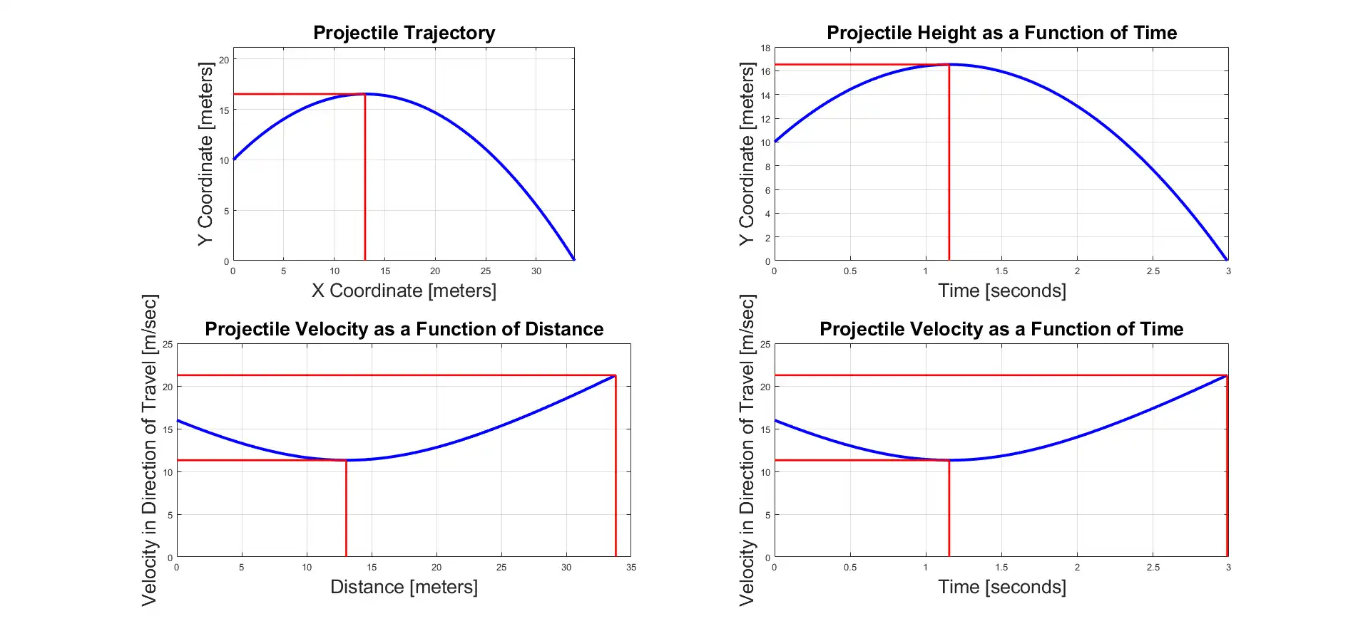
% Plot the location of the projectile.
hFigure = figure;
subplot(2, 2, 1);
plot(x, y, 'b-', 'LineWidth', 3);
grid on;
xlabel('X Coordinate [meters]', 'FontSize', fontSize);
ylabel('Y Coordinate [meters]', 'FontSize', fontSize);
title ('Projectile Trajectory', 'FontSize', fontSize)
% Make x and y have the same scale
% so one is not stretched out with respect to the other
% and the angles will look correct.
axis equal;
% Make x axis start at 0.
xl = xlim(); % Get current x axis limits
xlim([0, xl(end)]);	% Make bottom limit 0.
% Make y axis start at 0.
yl = ylim(); % Get current y axis limits
yl(2) = max(yl(2), yTop);
ylim([0, yl(2)]);	% Make bottom limit 0.
% Draw a red line from the x axis to the top
line([xTop, xTop], [0, yTop], 'Color', 'r', 'LineWidth', 2);
% Draw a red line from the y axis to the top
line([0, xTop], [yTop, yTop], 'Color', 'r', 'LineWidth', 2);

% Set up figure properties:
% Enlarge figure to full screen.
set(gcf, 'Units', 'Normalized', 'OuterPosition', [0, 0.1, 1, 0.9]);
% Get rid of tool bar and pulldown menus that are along top of figure.
% set(gcf, 'Toolbar', 'none', 'Menu', 'none');
% Give a name to the title bar.
set(gcf, 'Name', 'Projectile Trajectory Demo', 'NumberTitle', 'Off') 

% Plot the height of the projectile as a function of time.
subplot(2, 2, 2);
plot(t, y, 'b-', 'LineWidth', 3);
grid on;
xlabel('Time [seconds]', 'FontSize', fontSize);
ylabel('Y Coordinate [meters]', 'FontSize', fontSize);
title ('Projectile Height as a Function of Time', 'FontSize', fontSize)
% Draw a red line from the x axis to the top
line([tTop, tTop], [0, yTop], 'Color', 'r', 'LineWidth', 2);
% Draw a red line from the y axis to the top
line([0, tTop], [yTop, yTop], 'Color', 'r', 'LineWidth', 2);

% Plot the velocity as a function of distance.
subplot(2, 2, 3);
plot(x, velocity, 'b-', 'LineWidth', 3);
grid on;
xlabel('Distance [meters]', 'FontSize', fontSize);
ylabel('Velocity in Direction of Travel [m/sec]', 'FontSize', fontSize);
title ('Projectile Velocity as a Function of Distance', 'FontSize', fontSize)
% Draw a red line from the x axis to the top.
line([xTop, xTop], [0, vTop], 'Color', 'r', 'LineWidth', 2);
% Draw a red line from the x axis to the final.
line([xFinal, xFinal], [0, vFinal], 'Color', 'r', 'LineWidth', 2);
% Draw a red line from the y axis to the top.
line([0, xTop], [vTop, vTop], 'Color', 'r', 'LineWidth', 2);
% Draw a red line from the y axis to the final.
line([0, xFinal], [vFinal, vFinal], 'Color', 'r', 'LineWidth', 2);

% Plot the velocity as a function of time.
subplot(2, 2, 4);
plot(t, velocity, 'b-', 'LineWidth', 3);
grid on;
xlabel('Time [seconds]', 'FontSize', fontSize);
ylabel('Velocity in Direction of Travel [m/sec]', 'FontSize', fontSize);
title ('Projectile Velocity as a Function of Time', 'FontSize', fontSize)
% Draw a red line from the x axis to the top.
line([tTop, tTop], [0, vTop], 'Color', 'r', 'LineWidth', 2);
% Draw a red line from the x axis to the final.
line([tFinal, tFinal], [0, vFinal], 'Color', 'r', 'LineWidth', 2);
% Draw a red line from the y axis to the top.
line([0, tTop], [vTop, vTop], 'Color', 'r', 'LineWidth', 2);
% Draw a red line from the y axis to the final.
line([0, tFinal], [vFinal, vFinal], 'Color', 'r', 'LineWidth', 2);


%===========================================================================================================================================================
%========== REPORT FINDINGS TO USER ========================================================================================================================
%===========================================================================================================================================================
% Tell user the results
s1 = sprintf('The total time of travel is %f seconds.\n', tFinal);
s2 = sprintf('The maximum x coordinate is %f meters.\n', xFinal);
s3 = sprintf('The range (horizontal distance from launch site) is %f meters.\n', xFinal - x0);
s4 = sprintf('The x distance until the top is %f meters.\n', xTop);
s5 = sprintf('The max y height at the top is %f meters.\n', yTop);
s6 = sprintf('The time until the top is %f seconds.\n', tTop);
s7 = sprintf('The min velocity, which will be at the top, is %f m/s.\n', vTop);
s8 = sprintf('The max velocity, which will be at the end, is %f m/s.\n', vFinal);
message = sprintf('%s%s%s%s%s%s%s%s', s1, s2, s3, s4, s5, s6, s7, s8);
uiwait(helpdlg(message, 'Simulation Results'));
% close(hFigure);

%===========================================================================================================================================================
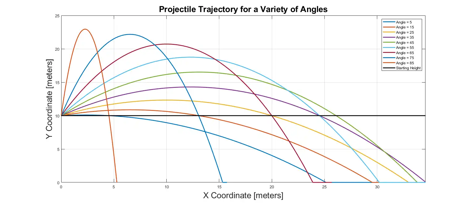
% PART 2 OF THE SIMULATION: TRAJECTORY FOR SEVERAL ANGLES.
% First find the max time of flight.  This will happen when the projectile is fired straight up and the angle is 90.
angle = 90;
% Get the components of velocity in the x and y directions.
v0x = v0*cosd(angle);
v0y = v0*sind(angle);

% Compute the distance along the y direction.  y = y0 + y_velocity_initial * time + (1/2)*g*time^2
% Now assume that the y value is zero when the projectile hits the ground.
% So we basically have a quadratic equation = = a*time^2 + b * time + c.
% y=0 (landed on the ground) at a time we'll call tFinal.
% To solve for tFinal we can use roots() to solve the quadratic equation.
a = (1/2) * g;
b = v0y;
c = y0;
tFinal = roots([a, b, c]);
tFinal = max(tFinal); % Take the positive value.
% Let's bring up a brand new figure.
hFig2 = figure();

% Let's make up a time vector going from 0 to tFinal rounded up to the next larger integer.
t = linspace(0, tFinal, 1000);
legends = {}; % Instantiate an empty cell for the angle legend.
counter = 1;
for angle = 5 : 10 : 90
	% Get the components of velocity in the x and y directions for this angle.
	v0x = v0*cosd(angle);
	v0y = v0*sind(angle);
	% Compute the distance along the x direction.  x = x0 + x_velocity * time.
	x = x0 + v0x * t;
	% Compute the distance along the y direction.  y = y0 + y_velocity_initial * time + (1/2)*g*time^2
	y = y0 + v0y * t + (1/2) * g * t .^ 2;
	% Clip y to zero because we assume the projectile stays on the ground when it hits.  
	% It does not penetrate and have a negative y.
	y(y < 0) = 0;
	indexHitGround = find(y > 0, 1, 'last');

	plot(x, y, '-', 'LineWidth', 2);
	hold on;
	legends{end+1} = sprintf('Angle = %d', angle);

% 	% Sort of "animate" it.
% 	if counter == 1
% 		% Set up figure properties:
% 		% Enlarge figure to full screen.
% 		set(gcf, 'Units', 'Normalized', 'OuterPosition', [0.1, 0.15, 0.8, 0.7]);
% 		% Get rid of tool bar and pulldown menus that are along top of figure.
% 		set(gcf, 'Toolbar', 'none', 'Menu', 'none');
% 		% Give a name to the title bar.
% 		set(gcf, 'Name', 'Projectile Trajectory Demo Part 2', 'NumberTitle', 'Off')
% 	end
% 
% 	drawnow;
% 	pause(.5);
	
	% Calculate the range in the x direction.
	xFinal(counter) = x(indexHitGround);
	counter = counter + 1;	
end
grid on;
xlabel('X Coordinate [meters]', 'FontSize', fontSize);
ylabel('Y Coordinate [meters]', 'FontSize', fontSize);
title ('Projectile Trajectory for a Variety of Angles', 'FontSize', fontSize)
% Draw a black line across the starting height.
line(xlim, [y0, y0], 'Color', 'k', 'LineWidth', 2);
% Add a lengend for the starting height line.
legends{end+1} = 'Starting Height';
legend(legends);
% Find the max xFinal and set the range of the graph to be that.
xlim([0, max(xFinal)]);

% Set up figure properties:
% Enlarge figure to full screen.
set(gcf, 'Units', 'Normalized', 'OuterPosition', [0.1, 0.15, 0.8, 0.7]);
% Get rid of tool bar and pulldown menus that are along top of figure.
% set(gcf, 'Toolbar', 'none', 'Menu', 'none');
% Give a name to the title bar.
set(gcf, 'Name', 'Projectile Trajectory Demo Part 2', 'NumberTitle', 'Off') 

Yes, but have you searched this forum? If you had, you would have seen lots of posts about projectiles where I attached a simulation program. See attached projectile demo. It lets you input lots of input parameters (height, angle, etc.) and computes practically everything you'd want to know about a projectile.

Not satisfied with the answer ?? ASK NOW