Introduction: Root Locus Controller Design

Contents

Closed-Loop Poles

The root locus of an (open-loop) transfer function  is a plot of the locations (locus) of all possible closed-loop poles with some parameter, often a proportional gain , varied between 0 and . The figure below shows a unity-feedback architecture, but the procedure is identical for any open-loop transfer function , even if some elements of the open-loop transfer function are in the feedback path.

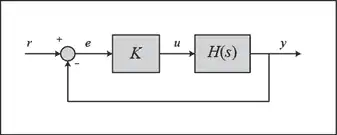
The closed-loop transfer function in this case is:

(1)

and thus the poles of the closed-loop system are values of  such that .

If we write , then this equation can be rewritten as:

(2)

(3)

Let  be the order of  and  be the order of  (the order of the polynomial corresponds to the highest power of ).

We will consider all positive values of . In the limit as , the poles of the closed-loop system are solutions of  (poles of ). In the limit as , the poles of the closed-loop system are solutions of  (zeros of ).

No matter our choice of , the closed-loop system has  poles, where  is the number of poles of the open-loop transfer function . The root locus then has  branches, each branch starts at a pole of  and approaches a zero of . If  has more poles than zeros (as is often the case),  and we say that  has zeros at infinity. In this case, the limit of  as  is zero. The number of zeros at infinity is , the number of open-loop poles minus the number of open-loop zeros, and is the number of branches of the root locus that go to "infinity" (asymptotes).

Since the root locus consists of the locations of all possible closed-loop poles, the root locus helps us choose the value of the gain  to achieve the type of performance we desire. If any of the selected poles are on the right-half complex plane, the closed-loop system will be unstable. The poles that are closest to the imaginary axis have the greatest influence on the closed-loop response, so even if a system has three or four poles, it may still behave similar to a second- or a first-order system, depending on the location(s) of the dominant pole(s).

Plotting the Root Locus of a Transfer Function

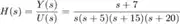
Consider an open-loop system which has a transfer function of

(4)

How do we design a feedback controller for the system using the root-locus method? Let's assume our design criteria are 5% overshoot and 1 second rise time. Create an m-file titled rl.m. Within this file, create the transfer function model and employ the rlocus command as follows:

s = tf('s');
sys = (s + 7)/(s*(s + 5)*(s + 15)*(s + 20));
rlocus(sys)
axis([-22 3 -15 15])

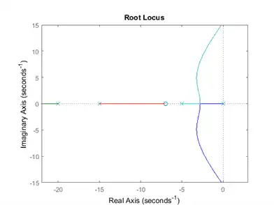
Choosing a Value of K from the Root Locus

The plot above shows all possible closed-loop pole locations for a pure proportional controller. In this case, not all of these closed-loop pole locations indicate satisfaction of our design criteria. To determine what part of the locus is acceptable, we can use the command sgrid(zeta,wn) to plot lines of constant damping ratio and natural frequency. Its two arguments are the damping ratio () and natural frequency () [these may be vectors if you want to look at a range of acceptable values]. In our problem, we need an overshoot less than 5% (which means a damping ratio  of greater than 0.7) and a rise time of 1 second (which means a natural frequency  greater than 1.8). Enter the following in the MATLAB command window:

zeta = 0.7;
wn = 1.8;
sgrid (zeta, wn)

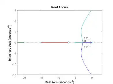
On the plot above, the two dotted lines at about a 45-degree angle indicate pole locations with  = 0.7; in between these lines, the poles will have  > 0.7 and outside of these lines  < 0.7. The semicircle indicates pole locations with a natural frequency  = 1.8; inside of the circle,  < 1.8 and outside of the circle  > 1.8.

Going back to our problem, to make the overshoot less than 5%, the poles have to be in between the two angled dotted lines, and to make the rise time shorter than 1 second, the poles have to be outside of the dotted semicircle. So now we know what part of the root locus, which possible closed-loop pole locations, satify the given requirements. All the poles in this location are in the left-half plane, so the closed-loop system will be stable.

From the plot above we see that there is part of the root locus inside the desired region. Therefore, in this case, we need only a proportional controller to move the poles to the desired region. You can use the rlocfind command in MATLAB to choose the desired poles on the locus:

[k,poles] = rlocfind(sys)

Click on the plot the point where you want the closed-loop pole to be. You may want to select the points indicated in the plot below to satisfy the design criteria.

Note that since the root locus may have more than one branch, when you select a pole, you also identify where other closed-loop poles are too, all for the same corresponding value of . Remember that these poles will affect the response too. From the plot above, we see that of the four poles selected (indicated by "+" signs), the two closest to the imaginary axis are in our desired region. Since these poles tend to dominate the response, we have some confidence that are desired requirements will be met for a proportional controller with this value of .

Closed-Loop Response

In order to verify the step response, you need to know the closed-loop transfer function. You could compute this using the rules of block diagram reduction, or let MATLAB do it for you (there is no need to enter a value for K if the rlocfind command was used):

K = 350;
sys_cl = feedback(K*sys,1)

sys_cl =
 
               350 s + 2450
  --------------------------------------
  s^4 + 40 s^3 + 475 s^2 + 1850 s + 2450
 
Continuous-time transfer function.

The two arguments to the function feedback are the transfer function in the forward path and the transfer function in the feedback path of the open-loop system. In this case, our system is unity feedback.

If you have a non-unity feedback situation, look at the help file for the MATLAB function feedback, which demonstrates how to find the closed-loop transfer function with a gain in the feedback path.

Checking the step response of the closed-loop system with the chosen value of :

step(sys_cl)

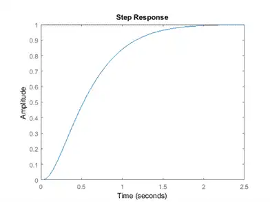
As we expected, this response has an overshoot less than 5% and a rise time less than 1 second.

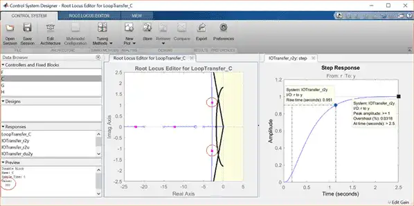
Using Control System Designer for Root Locus Design

Another way to complete what was done above is to use the interactive Control System Designer tool within MATLAB. Using the same model as above, we first define the plant, .

s = tf('s');
plant = (s + 7)/(s*(s + 5)*(s + 15)*(s + 20));

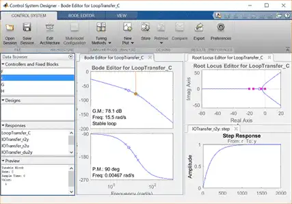
The controlSystemDesigner function can be used for analysis and design. In this case, we will focus on using the root locus as the design method to improve the step response of the closed-loop system. To begin, type the following into the MATLAB command window:

controlSystemDesigner(plant)

The following window should appear. You can also launch the GUI by going to the APPS tab and clicking on the app icon under Control System Design and Analysis. Here you can see the root locus plot, along with open-loop Bode plot, and the closed-loop step response plot for the given plant in unity feedback with a default controller of .

The next step is to add the design requirements to the Root Locus plot. This is done directly on the plot by right-clicking and selecting Design Requirements, New. Design requirements can be set for the Settling Time, the Percent Overshoot, the Damping Ratio, the Natural Frequency, or a Region Constraint.

Here, we will set the design requirements for the damping ratio and the natural frequency as was done previously with the sgrid command. Recall that the boundary of our requirements call for  = 0.7 and  = 1.8. Set these within the design requirements. On the plot, any area which is still white is an acceptable region for the closed-loop poles.

Zoom into the Root Locus by right-clicking on an axis and selecting Properties followed by the label Limits. Change the real-axis limits to -25 to 5 and the imaginary axis limits to -2.5 to 2.5.

Also, we can see the current values of some key parameters in the response. On the Step response plot, right-click on the plot and go to Characteristics and select Peak Response. Repeat for the characteristic Rise Time. There should now be two large dots on the screen indicating the values of these parameters. Click each of these dots to bring up a box with information.

Both plots should appear as shown here, once the Bode plot is closed:

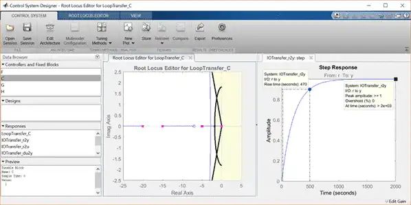
As the characteristics show on the Step response, the overshoot is acceptable, but the rise time is much too large. The pink boxes on the root locus show the corresponding closed-loop pole locations for the currently chosen control gain .

To fix this, we need to choose a new value for the gain . Similar to how we employed the rlocfind command, the gain of the controller can be changed directly on the root locus plot. Click and drag the pink box closest to the imaginary axis (at the origin) to the acceptable region of our root locus plot as shown below.

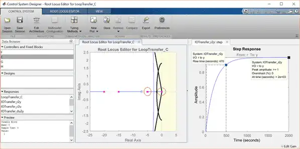
In the Preview box of the window, it can be seen that the loop gain has been changed to 360. Inspecting the closed-loop step response plot, both of our requirements are now met.